
FX Vol Surfaces#
Warning
FX volatility products in rateslib are not in stable status. Their API and/or object interactions may incur breaking changes in upcoming releases as they mature and other classes or pricing models may be added.
The rateslib.fx_volatility module includes classes for Smiles and Surfaces
which can be used to price FX Options and FX Option Strategies.
Create an FX Volatility Smile at a given expiry indexed by delta percent. |
|
Create an FX Volatility Surface parametrised by cross-sectional Smiles at different expiries. |
Introduction and FX Volatility Smiles#
The FXDeltaVolSmile is parametrised by a series of
(delta-index, vol) node points interpolated by a cubic spline. This interpolation is
automatically constructed with knot sequences that adjust to the number of given nodes:
Providing only one node, e.g. (0.5, 11.0), will create a constant volatility level, here at 11%.
Providing two nodes, e.g. (0.25, 8.0), (0.75, 10.0) will create a straight line gradient across the whole delta axis, here rising by 1% volatility every 0.25 in delta-index.
Providing more nodes (appropriately calibrated) will create a traditional smile shape with the mentioned interpolation structure.
An FXDeltaVolSmile must also be initialised with:
An
eval_datewhich serves the same purpose as the initial node point on a Curve, and indicates ‘today’.An
expiry, for which options priced with this Smile must have an equivalent expiry or errors will be raised.A
delta_typeso that its delta-index is well defined, and it can price different Instruments even if their delta types are different. I.e. A Smile defined by “forward” delta types can still price FXOptions defined with “spot” delta types due to appropriate mathematical conversions.
In [1]: smile = FXDeltaVolSmile(
   ...:     eval_date=dt(2000, 1, 1),
   ...:     expiry=dt(2000, 7, 1),
   ...:     nodes={
   ...:         0.25: 10.3,
   ...:         0.5: 9.1,
   ...:         0.75: 10.8
   ...:     },
   ...:     delta_type="forward"
   ...: )
   ...:

#  -->  smile.plot()
#  -->  smile.plot(x_axis="moneyness")

Constructing a Smile#
The following data describes Instruments to calibrate the EURUSD FX volatility surface on 7th May 2024. We will take a cross-section of this data, at the 3-week expiry (28th May 2024), and create an FXDeltaVolSmile.
Since EURUSD is not premium adjusted and the premium currency is USD we will match the Smile
with this definition and set it to a delta_type of ‘spot’, matching the market convention
of these quoted instruments. Since we have 5 calibrating instruments we require 5 degrees
of freedom.
In [2]: smile = FXDeltaVolSmile(
   ...:     nodes={
   ...:         0.10: 10.0,
   ...:         0.25: 10.0,
   ...:         0.50: 10.0,
   ...:         0.75: 10.0,
   ...:         0.90: 10.0,
   ...:     },
   ...:     eval_date=dt(2024, 5, 7),
   ...:     expiry=dt(2024, 5, 28),
   ...:     delta_type="spot",
   ...:     id="eurusd_3w_smile"
   ...: )
   ...:
The above Smile is initialised as a flat vol at 10%. In order to calibrate it we need to create the pricing instruments, given in the market prices data table.
Since these Instruments are multi-currency derivatives an FXForwards
framework also needs to be setup for pricing. We will do this simultaneously using other prevailing market data,
i.e. local currency interest rates at 3.90% and 5.32%, and an FX Swap rate at 8.85 points.
# Define the interest rate curves for EUR, USD and X-Ccy basis
In [3]: eureur = Curve({dt(2024, 5, 7): 1.0, dt(2024, 5, 30): 1.0}, calendar="tgt", id="eureur")
In [4]: eurusd = Curve({dt(2024, 5, 7): 1.0, dt(2024, 5, 30): 1.0}, id="eurusd")
In [5]: usdusd = Curve({dt(2024, 5, 7): 1.0, dt(2024, 5, 30): 1.0}, calendar="nyc", id="usdusd")
# Create an FX Forward market with spot FX rate data
In [6]: fxf = FXForwards(
...: fx_rates=FXRates({"eurusd": 1.0760}, settlement=dt(2024, 5, 9)),
...: fx_curves={"eureur": eureur, "usdusd": usdusd, "eurusd": eurusd},
...: )
...:
# Setup the Solver instrument calibration for rates Curves and vol Smiles
In [7]: option_args=dict(
...: pair="eurusd", expiry=dt(2024, 5, 28), calendar="tgt", delta_type="spot",
...: curves=[None, "eurusd", None, "usdusd"], vol="eurusd_3w_smile"
...: )
...:
In [8]: solver = Solver(
...: curves=[eureur, eurusd, usdusd, smile],
...: instruments=[
...: IRS(dt(2024, 5, 9), "3W", spec="eur_irs", curves="eureur"),
...: IRS(dt(2024, 5, 9), "3W", spec="usd_irs", curves="usdusd"),
...: FXSwap(dt(2024, 5, 9), "3W", pair="eurusd", curves=[None, "eurusd", None, "usdusd"]),
...: FXStraddle(strike="atm_delta", **option_args),
...: FXRiskReversal(strike=["-25d", "25d"], **option_args),
...: FXRiskReversal(strike=["-10d", "10d"], **option_args),
...: FXBrokerFly(strike=["-25d", "atm_delta", "25d"], **option_args),
...: FXBrokerFly(strike=["-10d", "atm_delta", "10d"], **option_args),
...: ],
...: s=[3.90, 5.32, 8.85, 5.493, -0.157, -0.289, 0.071, 0.238],
...: fx=fxf,
...: )
...:
SUCCESS: `func_tol` reached after 11 iterations (levenberg_marquardt), `f_val`: 7.709670586017593e-13, `time`: 0.1129s
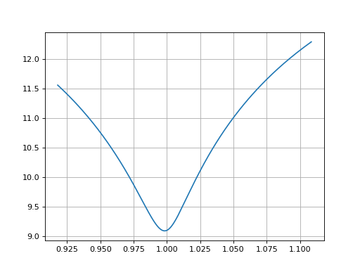
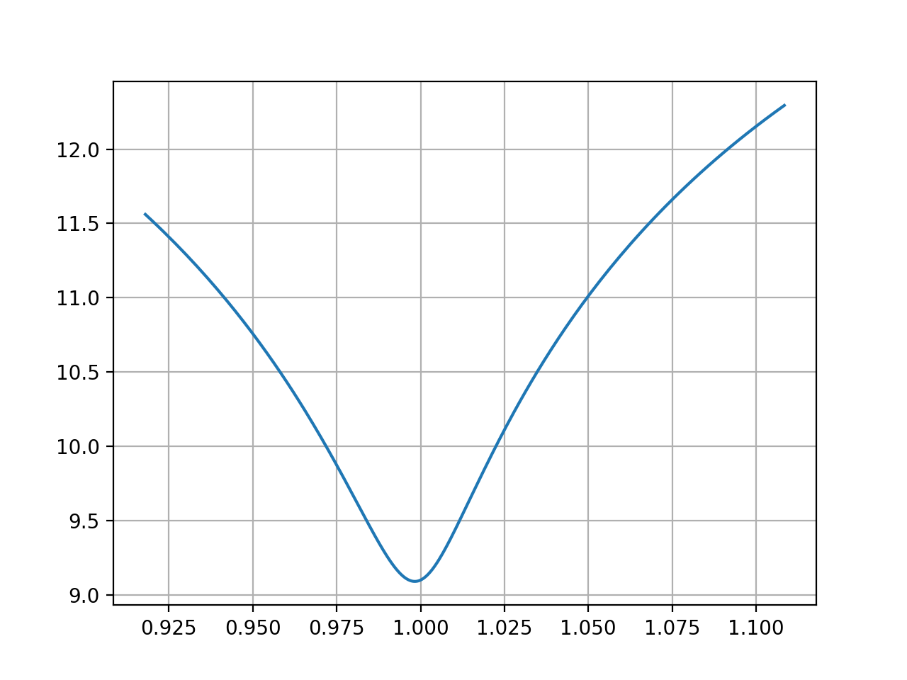
In [9]: smile.plot()
Out[9]:
(<Figure size 640x480 with 1 Axes>,
<Axes: >,
[<matplotlib.lines.Line2D at 0x11dc7f9d0>])
(Source code, png, hires.png, pdf)
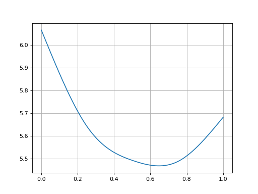
Rateslib Vol Smile#
FX Volatility Surfaces#
FX Surfaces in rateslib are collections of cross sectional FX Smiles where:
each cross-sectional Smile will represent a Smile at that explicit expiry,
the delta type and the delta indexes on each cross-sectional Smile are the same,
each Smile has its own calibrated node values,
Smiles for expiries that do not pre-exist are generated with an interpolation scheme that uses linear total variance, which is equivalent to flat-forward volatility
To demonstrate this, we will use an example adapted from Iain Clark’s Foreign Exchange Option Pricing: A Practitioner’s Guide.
The eval_date is fictionally assumed to be 3rd May 2009 and the FX spot rate is 1.34664,
and the continuously compounded EUR and USD rates are 1.0% and 0.4759..% respectively. With these
we will be able to closely match his values for option strikes.
# Setup the FXForward market...
In [10]: eur = Curve({dt(2009, 5, 3): 1.0, dt(2011, 5, 10): 1.0})

In [11]: usd = Curve({dt(2009, 5, 3): 1.0, dt(2011, 5, 10): 1.0})

In [12]: fxf = FXForwards(
   ....:     fx_rates=FXRates({"eurusd": 1.34664}, settlement=dt(2009, 5, 5)),
   ....:     fx_curves={"eureur": eur, "usdusd": usd, "eurusd": eur},
   ....: )
   ....:

In [13]: solver = Solver(
   ....:     curves=[eur, usd],
   ....:     instruments=[
   ....:         Value(dt(2009, 5, 4), curves=eur, metric="cc_zero_rate"),
   ....:         Value(dt(2009, 5, 4), curves=usd, metric="cc_zero_rate")
   ....:     ],
   ....:     s=[1.00, 0.4759550366220911],
   ....:     fx=fxf,
   ....: )
   ....:
SUCCESS: `func_tol` reached after 4 iterations (levenberg_marquardt), `f_val`: 5.204923799977582e-16, `time`: 0.0019s
His Table 4.2 is shown below, which outlines the delta type of the used instruments at their respective tenors, and the ATM-delta straddle, the 25-delta broker-fly and the 25-delta risk reversal market volatility prices.
In [14]: data = DataFrame(
   ....:     data = [["spot", 18.25, 0.95, -0.6], ["forward", 17.677, 0.85, -0.562]],
   ....:     index=["1y", "2y"],
   ....:     columns=["Delta Type", "ATM", "25dBF", "25dRR"],
   ....: )
   ....:

In [15]: data
Out[15]:
   Delta Type   ATM  25dBF  25dRR
1y       spot 18.25   0.95  -0.60
2y    forward 17.68   0.85  -0.56
Constructing a Surface#
We will now create a Surface that will be calibrated by those given rates. The Surface is initialised at a flat 18% volatility.
In [16]: surface = FXDeltaVolSurface(
   ....:     eval_date=dt(2009, 5, 3),
   ....:     delta_indexes=[0.25, 0.5, 0.75],
   ....:     expiries=[dt(2010, 5, 3), dt(2011, 5, 3)],
   ....:     node_values=np.ones((2, 3))* 18.0,
   ....:     delta_type="forward",
   ....:     id="surface",
   ....: )
   ....:
The calibration of the Surface requires a Solver that will iterate and update the surface node values until convergence with the given instrument rates.
Note
The Surface is parametrised by a ‘forward’ delta type but that the 1Y Instruments use ‘spot’. Internally this is all handled appropriately with necessary conversions, but it is the users responsibility to label the Surface and Instrument with the correct types. As Clark and others highlight “failing to take [correct delta types] into account introduces a mismatch - large enough to be relevant for calibration and pricing, but small enough that it may not be noticed at first”. Parametrising the Surface with a ‘forward’ delta type is the recommended choice because it is more standardised and the configuration of which delta types to use for the Instruments can be a separate consideration.
For performance reasons it is recommended to match unadjusted delta type Surfaces with calibrating Instruments that also have unadjusted delta types. And vice versa with premium adjusted delta types. However, rateslib has internal root solvers which can handle these cross-delta type specifications, although it degrades the performance of the Solver because the calculations are more difficult. Mixing ‘spot’ and ‘forward’ is not a difficult distinction to refactor and that does not cause performance degradation.
In [17]: fx_args_0 = dict(
   ....:     pair="eurusd",
   ....:     curves=[None, eur, None, usd],
   ....:     expiry=dt(2010, 5, 3),
   ....:     delta_type="spot",
   ....:     vol="surface",
   ....: )
   ....:

In [18]: fx_args_1 = dict(
   ....:     pair="eurusd",
   ....:     curves=[None, eur, None, usd],
   ....:     expiry=dt(2011, 5, 3),
   ....:     delta_type="forward",
   ....:     vol="surface",
   ....: )
   ....:

In [19]: solver = Solver(
   ....:     surfaces=[surface],
   ....:     instruments=[
   ....:         FXStraddle(strike="atm_delta", **fx_args_0),
   ....:         FXBrokerFly(strike=["-25d", "atm_delta", "25d"], **fx_args_0),
   ....:         FXRiskReversal(strike=["-25d", "25d"], **fx_args_0),
   ....:         FXStraddle(strike="atm_delta", **fx_args_1),
   ....:         FXBrokerFly(strike=["-25d", "atm_delta", "25d"], **fx_args_1),
   ....:         FXRiskReversal(strike=["-25d", "25d"], **fx_args_1),
   ....:     ],
   ....:     s=[18.25, 0.95, -0.6, 17.677, 0.85, -0.562],
   ....:     fx=fxf,
   ....: )
   ....:
SUCCESS: `func_tol` reached after 10 iterations (levenberg_marquardt), `f_val`: 3.638632286230408e-12, `time`: 0.0895s
The table below is rateslib’s replicated calculations of Clark’s Table 4.5. Note that due to:
using a different parametric form for Smiles (i.e. a natural cubic spline),
inferring his FX forwards market rates,
and not necessarily knowing the exact dates and holiday calendars of his example,
this produces minor deviations from his calculated values.
In [20]: with option_context("display.float_format", lambda x: '%.4f' % x):
   ....:     print(data2)
   ....:
            25d Put  ATM Put  25d Call
(1y, k)      1.1969   1.3620    1.5492
(1y, vol)   19.5170  18.2500   18.9108
(18m, k)     1.1728   1.3684    1.5968
(18m, vol)  19.0414  17.8679   18.4645
(2y, k)      1.1537   1.3747    1.6393
(2y, vol)   18.8030  17.6770   18.2410
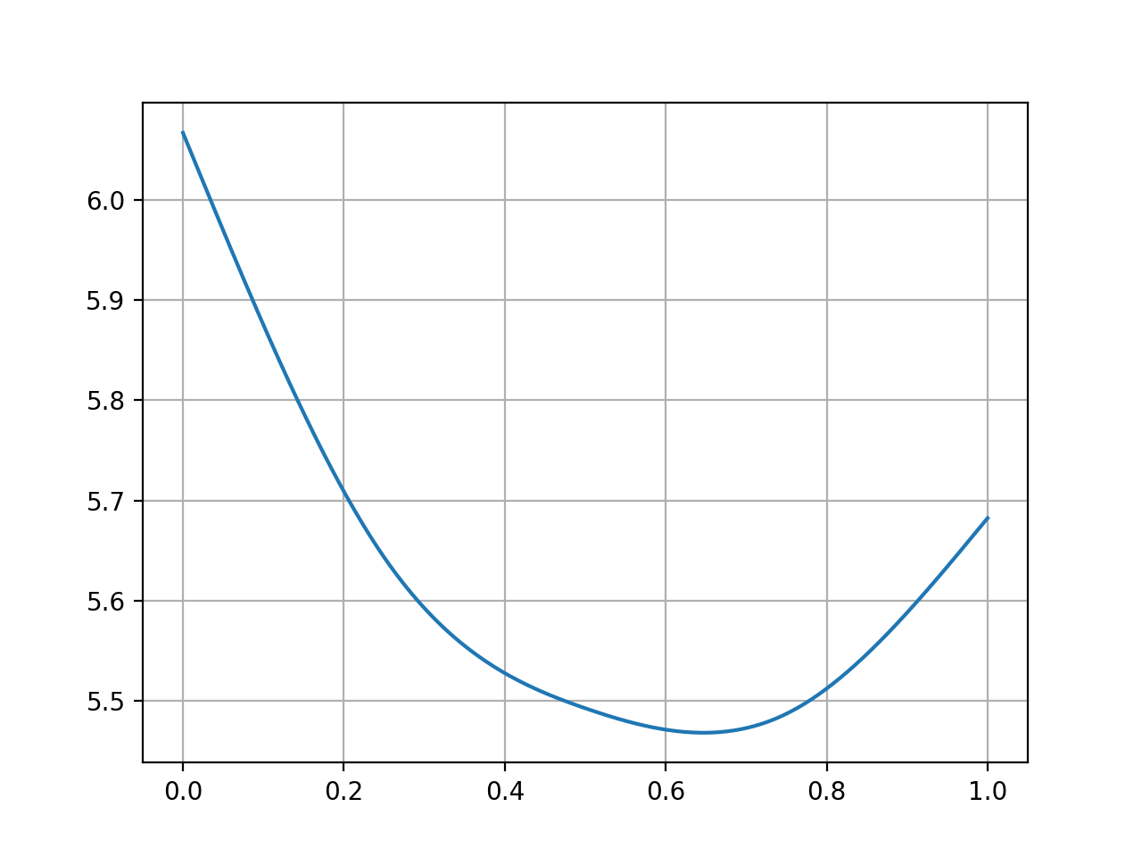
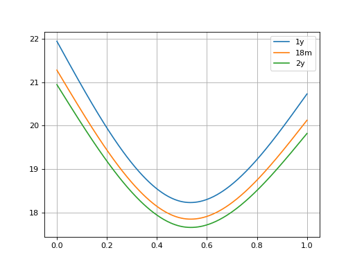
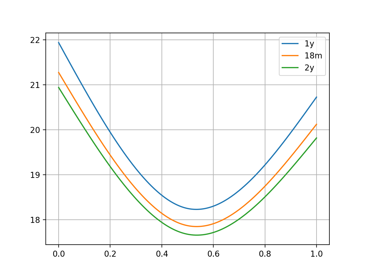
Plotting#
Three relevant cross-sectional Smiles from above are plotted.
In [21]: sm12 = surface.smiles[0]

In [22]: sm18 = surface.get_smile(dt(2010, 11, 3))

In [23]: sm24 = surface.smiles[1]

In [24]: sm12.plot(comparators=[sm18, sm24], labels=["1y", "18m", "2y"])
Out[24]:
(<Figure size 640x480 with 1 Axes>,
 <Axes: >,
 [<matplotlib.lines.Line2D at 0x11ddb5e50>,
  <matplotlib.lines.Line2D at 0x11ddb5f90>,
  <matplotlib.lines.Line2D at 0x11ddb60d0>])
(Source code, png, hires.png, pdf)

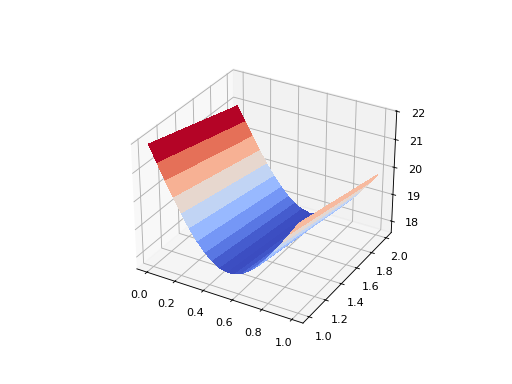
Alternative a 3D surface plot can also be shown.
In [25]: surface.plot()
Out[25]: (<Figure size 640x480 with 1 Axes>, <Axes3D: >, None)
(Source code, png, hires.png, pdf)
