
FX Volatility Surface Temporal Interpolation#
[1]:
from rateslib import *
from pandas import Series
import matplotlib.pyplot as plt
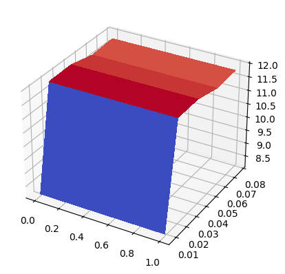
The default FXDeltaVolSurface is constructed with parametrised cross-sectional FXDeltaVolSmiles. The temporal interpolation method determines a delta-node between the two surrounding Smiles using linear total variance, which has been shown (see Clark: FX Option Pricing) to be equivalent to flat forward volatility within the interval.
Consider Table 4.7 of that same publication, Clark: FX Option Pricing. To replicate the data there we will create a Surface here which has flat line Smiles (i.e. there is just one volatility datapoint at each expiry) in the following way:
[2]:
fxvs = FXDeltaVolSurface(
    expiries=[
        dt(2024, 2, 12), # Spot
        dt(2024, 2, 16), # 1W
        dt(2024, 2, 23), # 2W
        dt(2024, 3, 1), # 3W
        dt(2024, 3, 8), # 4W
    ],
    delta_indexes=[0.5],
    node_values=[[8.15], [11.95], [11.97], [11.75], [11.80]],
    eval_date=dt(2024, 2, 9),
    delta_type="forward",
)
[3]:
fxvs.plot()
[3]:
(<Figure size 640x480 with 1 Axes>, <Axes3D: >, None)
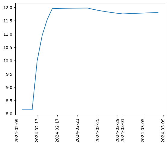
In the time/expiry dimension we will plot the volatility as measured for every calendar day expiry for the four weeks
[4]:
cal = get_calendar("all")
x, y = [], []
for date in cal.cal_date_range(dt(2024, 2, 10), dt(2024, 3, 8)):
    x.append(date)
    y.append(fxvs.get_smile(date).nodes[0.5])

fig, ax = plt.subplots(1,1)
plt.xticks(rotation=90)
ax.plot(x,y)
[4]:
[<matplotlib.lines.Line2D at 0x10a80ac10>]
Using Weights#
The comment in the publication is that markets do not assign volatility to calendar days when the market is closed. In this section we will provide weights that manipulate the forward volatility and align with table 4.7.
Date |
Weight |
Volatility to Expiry |
|---|---|---|
10 Feb ‘24 |
0.0 |
0.0 |
11 Feb ‘24 |
0.0 |
0.0 |
12 Feb ‘24 |
1.0 |
8.15 |
13 Feb ‘24 |
1.0 |
9.99 |
14 Feb ‘24 |
1.0 |
10.95 |
15 Feb ‘24 |
1.0 |
11.54 |
16 Feb ‘24 |
1.0 |
11.95 |
17 Feb ‘24 |
0.0 |
11.18 |
18 Feb ‘24 |
0.0 |
10.54 |
19 Feb ‘24 |
1.0 |
10.96 |
20 Feb ‘24 |
1.0 |
11.29 |
21 Feb ‘24 |
1.0 |
11.56 |
22 Feb ‘24 |
1.0 |
11.78 |
23 Feb ‘24 |
1.0 |
11.97 |
24 Feb ‘24 |
0.0 |
11.56 |
25 Feb ‘24 |
0.0 |
11.20 |
26 Feb ‘24 |
1.0 |
11.34 |
27 Feb ‘24 |
1.0 |
11.46 |
28 Feb ‘24 |
1.0 |
11.57 |
29 Feb ‘24 |
1.0 |
11.66 |
1 Mar ‘24 |
1.0 |
11.75 |
2 Mar ‘24 |
0.0 |
11.48 |
3 Mar ‘24 |
0.0 |
11.23 |
4 Mar ‘24 |
1.0 |
11.36 |
5 Mar ‘24 |
1.0 |
11.49 |
6 Mar ‘24 |
1.0 |
11.60 |
7 Mar ‘24 |
1.0 |
11.70 |
8 Mar ‘24 |
1.0 |
11.80 |
9 Mar ‘24 |
0.0 |
11.59 |
We can use the calendar methods in rateslib to create an indexed Series with zero weights where we want to have them.
[5]:
# Use a generic business day calendar to find the weekends
cal = get_calendar("bus")
weekends = [
    _  for _ in cal.cal_date_range(dt(2024, 2, 9), dt(2024, 3, 11))
    if _ not in cal.bus_date_range(dt(2024, 2, 9), dt(2024, 3, 11))
]
weights = Series(0.0, index=weekends)
weights
[5]:
2024-02-10    0.0
2024-02-11    0.0
2024-02-17    0.0
2024-02-18    0.0
2024-02-24    0.0
2024-02-25    0.0
2024-03-02    0.0
2024-03-03    0.0
2024-03-09    0.0
2024-03-10    0.0
dtype: float64
Now we will rebuild an FXDeltaVolSurface and plot the difference to before.
[6]:
fxvs_2 = FXDeltaVolSurface(
    expiries=[
        dt(2024, 2, 12), # Spot
        dt(2024, 2, 16), # 1W
        dt(2024, 2, 23), # 2W
        dt(2024, 3, 1), # 3W
        dt(2024, 3, 8), # 4W
    ],
    delta_indexes=[0.5],
    node_values=[[8.15], [11.95], [11.97], [11.75], [11.80]],
    eval_date=dt(2024, 2, 9),
    delta_type="forward",
    weights=weights,
)
[7]:
cal = get_calendar("all")
x, y, y2 = [], [], []
for date in cal.cal_date_range(dt(2024, 2, 10), dt(2024, 3, 8)):
    x.append(date)
    y.append(fxvs.get_smile(date).nodes[0.5])
    y2.append(fxvs_2.get_smile(date).nodes[0.5])

fig, ax = plt.subplots(1,1)
plt.xticks(rotation=90)
ax.plot(x,y, label="excl. weights")
ax.plot(x,y2, label="incl. weights")
ax.plot([dt(2024, 2, 12), dt(2024, 2, 16), dt(2024, 2, 23), dt(2024, 3, 1), dt(2024, 3, 8)],
        [8.15, 11.95, 11.97, 11.75, 11.80],
        "o", label="benchmarks"
       )
ax.legend()
[7]:
<matplotlib.legend.Legend at 0x10a64a660>
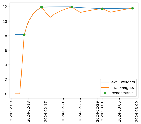
We observe the familiar sawtooth pattern that is frequently observed in short dated FX market vol.