
CreditImpliedCurve#
- class rateslib.curves.CreditImpliedCurve(risk_free=NoInput.blank, credit=NoInput.blank, hazard=NoInput.blank, id=NoInput.blank)#
Bases:
_BaseCurveImply a
_BaseCurvefrom credit components.Warning
This class is in beta status as of v2.1.0
- Parameters:
risk_free (_BaseCurve, optional) – The known risk free curve. If not given will be the implied curve.
credit (_BaseCurve, optional) – The known credit curve. If not given will be the implied curve.
hazard (_BaseCurve, optional) – The known hazard curve. If not given will be the implied curve.
Notes
A risk free, credit or hazard curve will be implied from the other known, provided curves.
This class is a wrapper for a
CompositeCurvewhere the two known curves are added and multiplied by the appropriate recovery rate, obtained from the_CurveMeta(either from thehazardcurve or thecreditcurve in that order of precedence) to derive the third.In traditional papers, such as Duffie and Singleton (1999), the credit DF is expressed relative to a risk free and hazard process. I.e.
\[exp \left ( \int_0^T -r_f(t) - (1-R)\lambda(t) .dt \right ) = exp \left ( \int_0^T -r_c(t) .dt \right )\]where \(r_f\) is the instantaneous risk free rate, \(r_c\) the instantaneous credit rate and \(\lambda\) the hazard intensity process.
In an approximation rateslib converts these to discrete overnight rate equivalents and implies the curves as follows under rate vector addition:
Credit curve rates: \(r_f(t) + (1-R)\lambda(t)\)
Hazard curve rates: \(\frac{r_c(t) - r_f(t)}{1-R}\)
Risk free rates: \(r_c(t) - (1-R)\lambda(t)\)
Example
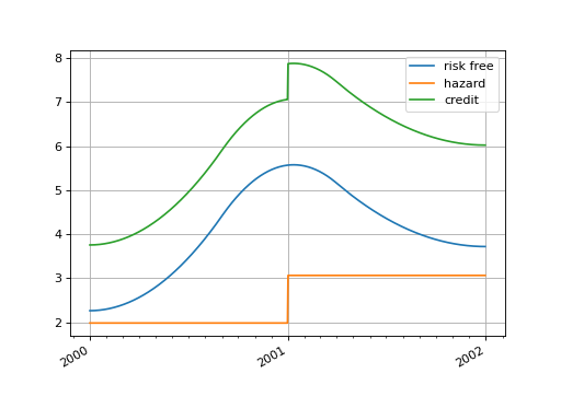
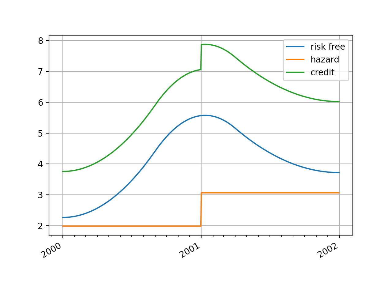
Given the following risk free curve and hazard curve, a credit curve is implied.
In [1]: from rateslib.curves import CreditImpliedCurve

In [2]: risk_free = Curve(
   ...:     nodes={dt(2000, 1, 1): 1.0, dt(2000, 9, 1): 0.98, dt(2001, 4, 1): 0.95, dt(2002, 1, 1): 0.92},
   ...:     interpolation="spline",
   ...: )
   ...:

In [3]: hazard = Curve(
   ...:     nodes={dt(2000, 1, 1): 1.0, dt(2001, 1, 1): 0.98, dt(2002, 1, 1): 0.95},
   ...:     credit_recovery_rate=0.25,
   ...: )
   ...:

In [4]: credit = CreditImpliedCurve(risk_free=risk_free, hazard=hazard)

In [5]: risk_free.plot("1b", comparators=[hazard, credit], labels=["risk free", "hazard", "credit"])
Out[5]:
(<Figure size 640x480 with 1 Axes>,
 <Axes: >,
 [<matplotlib.lines.Line2D at 0x110966660>,
  <matplotlib.lines.Line2D at 0x1109667b0>,
  <matplotlib.lines.Line2D at 0x110966900>])
(
Source code,png,hires.png,pdf)
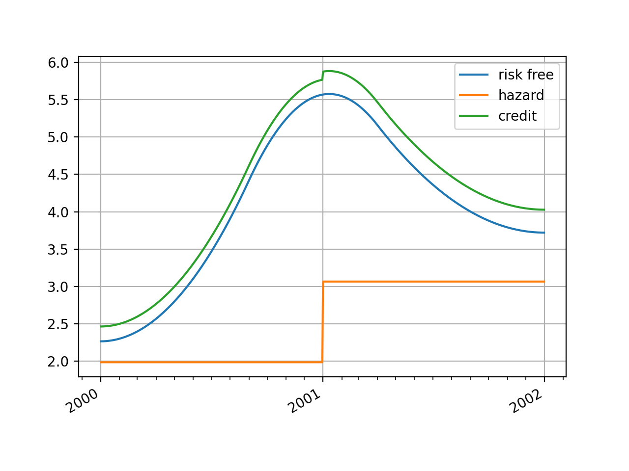
These associations are dynamic so changes to any of the curves will naturally update the
CreditImpliedCurve.In [6]: hazard.update_meta("credit_recovery_rate", 0.90) In [7]: risk_free.plot("1b", comparators=[hazard, credit], labels=["risk free", "hazard", "credit"]) Out[7]: (<Figure size 640x480 with 1 Axes>, <Axes: >, [<matplotlib.lines.Line2D at 0x11000cd70>, <matplotlib.lines.Line2D at 0x11000cec0>, <matplotlib.lines.Line2D at 0x11000d010>])
(
Source code,png,hires.png,pdf)
Attributes Summary
Int in {0,1,2} describing the AD order associated with the Curve.
A str identifier to name the Curve used in
Solvermappings.An instance of
_CurveInterpolator.An instance of
_CurveMeta.An instance of
_CurveNodes.The wrapped
CompositeCurvefor making calculations.Methods Summary
copy()Create an identical copy of the curve object.
index_value(index_date, index_lag[, ...])Calculate the accrued value of the index from the
index_base.plot(tenor[, right, left, comparators, ...])Plot given forward tenor rates from the curve.
plot_index([right, left, comparators, ...])Plot given index values on a Curve.
rate(effective[, termination, modifier, ...])Calculate the rate on the Curve using DFs.
roll(tenor[, id])Create a
RolledCurve: translating the rate space of Self in time.shift(spread[, id])Create a
ShiftedCurve: moving Self vertically in rate space.translate(start[, id])Create a
TranslatedCurve: maintaining an identical rate space, but moving the initial node date forwards in time.Attributes Documentation
- ad#
Int in {0,1,2} describing the AD order associated with the Curve.
- interpolator#
An instance of
_CurveInterpolator.
- meta#
An instance of
_CurveMeta.
- nodes#
An instance of
_CurveNodes.
- obj#
The wrapped
CompositeCurvefor making calculations.
Methods Documentation
- copy()#
Create an identical copy of the curve object.
- Return type:
Self
- index_value(index_date, index_lag, index_method=IndexMethod.Curve)#
Calculate the accrued value of the index from the
index_base.This method will raise if performed on a ‘values’ type Curve.
- Parameters:
index_date (datetime) – The reference date for which the index value will be returned.
index_lag (int) – The number of months by which to lag the index when determining the value.
index_method (IndexMethod or str in {"curve", "monthly", "daily"}) – The interpolation method for returning the index value. Monthly returns the index value for the start of the month and daily returns a value based on the interpolation between nodes (which is recommended “linear_index) for
InflationCurve.
- Return type:
Notes
The interpolation methods function as follows:
“curve”: will raise if the requested
index_lagdoes not match the lag attributed to the Curve. In the case theindex_lagmatches, then the index value for any date is derived via the implied interpolation for the discount factors of the Curve.\[I_v(m) = \frac{I_b}{v(m)}\]“monthly”: For any date, m, uses the “curve” method having adjusted m in two ways. Firstly it deducts a number of months equal to \(L - L_c\), where L is the given
index_lagand \(L_c\) is the index lag of the Curve. And the day of the month is set to 1.\[\begin{split}&I^{monthly}_v(m) = I_v(m_adj) \\ &\text{where,} \\ &m_adj = Date(Year(m), Month(m) - L + L_c, 1) \\\end{split}\]“daily”: For any date, m, with a given
index_lagperforms calendar day interpolation on surrounding “monthly” values.\[\begin{split}&I^{daily}_v(m) = I^{monthly}_v(m) + \frac{Day(m) - 1}{n} \left ( I^{monthly}_v(m_+) - I^{monthly}_v(m) \right ) \\ &\text{where,} \\ &m_+ = \text{Any date in the month following, }m &n = \text{Calendar days in, } Month(m)\end{split}\]
Examples
The SWESTR rate, for reference value date 6th Sep 2021, was published as 2.375% and the RFR index for that date was 100.73350964. Below we calculate the value that was published for the RFR index on 7th Sep 2021 by the Riksbank.
In [8]: index_curve = Curve(
   ...:     nodes={
   ...:         dt(2021, 9, 6): 1.0,
   ...:         dt(2021, 9, 7): 1 / (1 + 2.375/36000)
   ...:     },
   ...:     index_base=100.73350964,
   ...:     convention="Act360",
   ...:     index_lag=0,
   ...: )
   ...:

In [9]: index_curve.rate(dt(2021, 9, 6), "1d")
Out[9]: 2.3750000000015703

In [10]: index_curve.index_value(dt(2021, 9, 7), 0)
Out[10]: 100.7401552534832
- plot(tenor, right=NoInput.blank, left=NoInput.blank, comparators=NoInput.blank, difference=False, labels=NoInput.blank)#
Plot given forward tenor rates from the curve. See notes.
- Parameters:
tenor (str) – The tenor of the forward rates to plot, e.g. “1D”, “3M”.
right (datetime or str, optional) – The right bound of the graph. If given as str should be a tenor format defining a point measured from the initial node date of the curve. Defaults to the final node of the curve minus the
tenor.left (datetime or str, optional) – The left bound of the graph. If given as str should be a tenor format defining a point measured from the initial node date of the curve. Defaults to the initial node of the curve.
comparators (list[Curve]) – A list of curves which to include on the same plot as comparators.
difference (bool) – Whether to plot as comparator minus base curve or outright curve levels in plot. Default is False.
labels (list[str]) – A list of strings associated with the plot and comparators. Must be same length as number of plots.
- Returns:
(fig, ax, line)
- Return type:
Matplotlib.Figure, Matplotplib.Axes, Matplotlib.Lines2D
Notes
This function plots single-period, simple interest curve rates, which are defined as:
\[1 + r d = \frac{v_{start}}{v_{end}}\]where d is the day count fraction determined using the
conventionassociated with the Curve.This function does not plot swap rates, which is impossible since the Curve object contains no information regarding the parameters of the ‘swap’ (e.g. its frequency or its convention etc.). If
tenorslonger than one year are sought results may start to deviate from those one might expect. See Issue 246.
- plot_index(right=NoInput.blank, left=NoInput.blank, comparators=NoInput.blank, difference=False, labels=NoInput.blank, interpolation='curve')#
Plot given index values on a Curve.
- Parameters:
right (datetime or str, optional) – The right bound of the graph. If given as str should be a tenor format defining a point measured from the initial node date of the curve. Defaults to the final node of the curve minus the
tenor.left (datetime or str, optional) – The left bound of the graph. If given as str should be a tenor format defining a point measured from the initial node date of the curve. Defaults to the initial node of the curve.
comparators (list[Curve]) – A list of curves which to include on the same plot as comparators.
difference (bool) – Whether to plot as comparator minus base curve or outright curve levels in plot. Default is False.
labels (list[str]) – A list of strings associated with the plot and comparators. Must be same length as number of plots.
interpolation (str in {"curve", "daily", "monthly"}) – The type of index interpolation method to use.
- Returns:
(fig, ax, line)
- Return type:
Matplotlib.Figure, Matplotplib.Axes, Matplotlib.Lines2D
- rate(effective, termination=NoInput.blank, modifier=NoInput.inherit, float_spread=NoInput.blank, spread_compound_method=NoInput.blank)#
Calculate the rate on the Curve using DFs.
If rates are sought for dates prior to the initial node of the curve None will be returned.
- Parameters:
effective (datetime) – The start date of the period for which to calculate the rate.
termination (datetime or str) – The end date of the period for which to calculate the rate.
modifier (str, optional) – The day rule if determining the termination from tenor. If False is determined from the Curve modifier.
float_spread (float, optional) – A float spread can be added to the rate in certain cases.
spread_compound_method (str in {"none_simple", "isda_compounding"}) – The method if adding a float spread. If “none_simple” is used this results in an exact calculation. If “isda_compounding” or “isda_flat_compounding” is used this results in an approximation.
- Return type:
Notes
Calculating rates from a curve implies that the conventions attached to the specific index, e.g. USD SOFR, or GBP SONIA, are applicable and these should be set at initialisation of the
Curve. Thus, the convention used to calculate therateis taken from theCurvefrom whichrateis called.modifieris only used if a tenor is given as the termination.Major indexes, such as legacy IBORs, and modern RFRs typically use a
conventionwhich is either “Act365F” or “Act360”. These conventions do not need additional parameters, such as the termination of a leg, the frequency or a leg or whether it is a stub to calculate a DCF.Adding Floating Spreads
An optimised method for adding floating spreads to a curve rate is provided. This is quite restrictive and mainly used internally to facilitate other parts of the library.
When
spread_compound_methodis “none_simple” the spread is a simple linear addition.When using “isda_compounding” or “isda_flat_compounding” the curve is assumed to be comprised of RFR rates and an approximation is used to derive to total rate.
Examples
In [11]: curve_act365f = Curve(
   ....:     nodes={
   ....:         dt(2022, 1, 1): 1.0,
   ....:         dt(2022, 2, 1): 0.98,
   ....:         dt(2022, 3, 1): 0.978,
   ....:     },
   ....:     convention='Act365F'
   ....: )
   ....:

In [12]: curve_act365f.rate(dt(2022, 2, 1), dt(2022, 3, 1))
Out[12]: 2.6657902424774402
Using a different convention will result in a different rate:
In [13]: curve_act360 = Curve(
   ....:     nodes={
   ....:         dt(2022, 1, 1): 1.0,
   ....:         dt(2022, 2, 1): 0.98,
   ....:         dt(2022, 3, 1): 0.978,
   ....:     },
   ....:     convention='Act360'
   ....: )
   ....:

In [14]: curve_act360.rate(dt(2022, 2, 1), dt(2022, 3, 1))
Out[14]: 2.6292725679229547
- roll(tenor, id=NoInput.blank)#
Create a
RolledCurve: translating the rate space of Self in time.For examples see the documentation for
RolledCurve.- Parameters:
tenor (datetime, str or int) – The measure of time by which to translate the curve through time.
id (str, optional) – Set the id of the returned curve.
- Return type:
- shift(spread, id=NoInput.blank)#
Create a
ShiftedCurve: moving Self vertically in rate space.For examples see the documentation for
ShiftedCurve.- Parameters:
- Return type:
- translate(start, id=NoInput.blank)#
Create a
TranslatedCurve: maintaining an identical rate space, but moving the initial node date forwards in time.For examples see the documentation for
TranslatedCurve.- Parameters:
start (datetime) – The new initial node date for the curve. Must be after the original initial node date.
id (str, optional) – Set the id of the returned curve.
- Return type: