
LineCurve#
- class rateslib.curves.LineCurve(*args, **kwargs)#
Bases:
_WithMutability,_BaseCurveA
_BaseCurvewith value parametrisation at given node dates with interpolation.- Parameters:
nodes (dict[datetime: float]) – Parameters of the curve denoted by a node date and a corresponding value at that point.
interpolation (str in {"log_linear", "linear"} or callable) – The interpolation used in the non-spline section of the curve. That is the part of the curve between the first node in
nodesand the first knot int. If a callable, this allows a user-defined interpolation scheme, and this must have the signaturemethod(date, nodes), wheredateis the datetime whose DF will be returned andnodesis as above and is passed to the callable.t (list[datetime], optional) – The knot locations for the B-spline cubic interpolation section of the curve. If None all interpolation will be done by the method specified in
interpolation.endpoints (str or list, optional) – The left and right endpoint constraint for the spline solution. Valid values are in {“natural”, “not_a_knot”}. If a list, supply the left endpoint then the right endpoint.
id (str, optional, set by Default) – The unique identifier to distinguish between curves in a multi-curve framework. convention : str, optional, set by Default The convention of the curve for determining rates. Please see
dcf()for all available options.convention (str, optional, set by Default) – The convention of the curve for determining rates. Please see
dcf()for all available options.modifier (str, optional) – The modification rule, in {“F”, “MF”, “P”, “MP”}, for determining rates when input as a tenor, e.g. “3M”.
calendar (Cal, UnionCal, NamedCal, str, optional) – The holiday calendar object to use. If str, looks up named calendar from static data. Used for determining rates.
ad (int in {0, 1, 2}, optional) – Sets the automatic differentiation order. Defines whether to convert node values to float,
DualorDual2. It is advised against using this setting directly. It is mainly used internally.
Notes
The arguments
index_base,index_lag, andcollateralavailable onCurveare not used by, or relevant for, aLineCurve.This curve type is value based and it is parametrised by a set of (date, value) pairs set as
nodes. The initial node date of the curve is defined to be today, and can take a general value. The initial value will be affected by aSolver.Note
This curve type can only ever be used for forecasting rates and projecting cashflow calculations. It cannot be used to discount cashflows becuase it is not DF based and there is no mathematical one-to-one conversion available to imply DFs.
Intermediate values are determined through
interpolation. If local interpolation is adopted a value for an arbitrary date is dependent only on its immediately neighbouring nodes via the interpolation routine. Available options are:“linear” (default for this curve type)
“log_linear” (useful for values that exponential, e.g. stock indexes or GDP)
“spline”
“flat_forward”, (useful for replicating a DF based log-linear type curve)
“flat_backward”,
And also the following which are not recommended for this curve type:
“linear_index”
“linear_zero_rate”,
Spline Interpolation
Global interpolation in the form of a cubic spline is also configurable with the parameters
t, andendpoints. Setting aninterpolationof “spline” is syntactic sugar for automatically determining the most obvious knot sequencetto use all specified node dates. See splines for instruction of knot sequence calibration.If the knot sequence is provided directly then any dates prior to the first knot date in
twill be determined through the local interpolation method. This allows for mixed interpolation.This curve type cannot return arbitrary tenor rates. It will only return a single value which is applicable to that date. It is recommended to review RFR and IBOR Indexing to ensure indexing is done in a way that is consistent with internal instrument configuration.
Examples
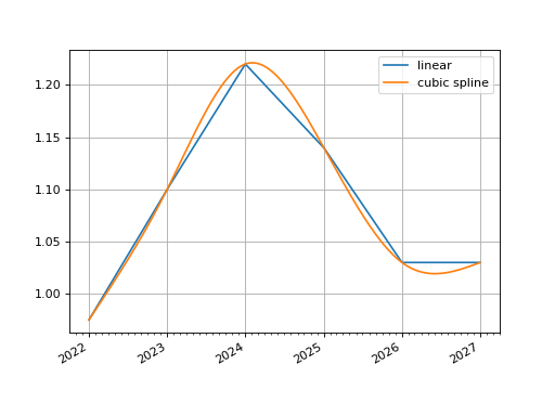
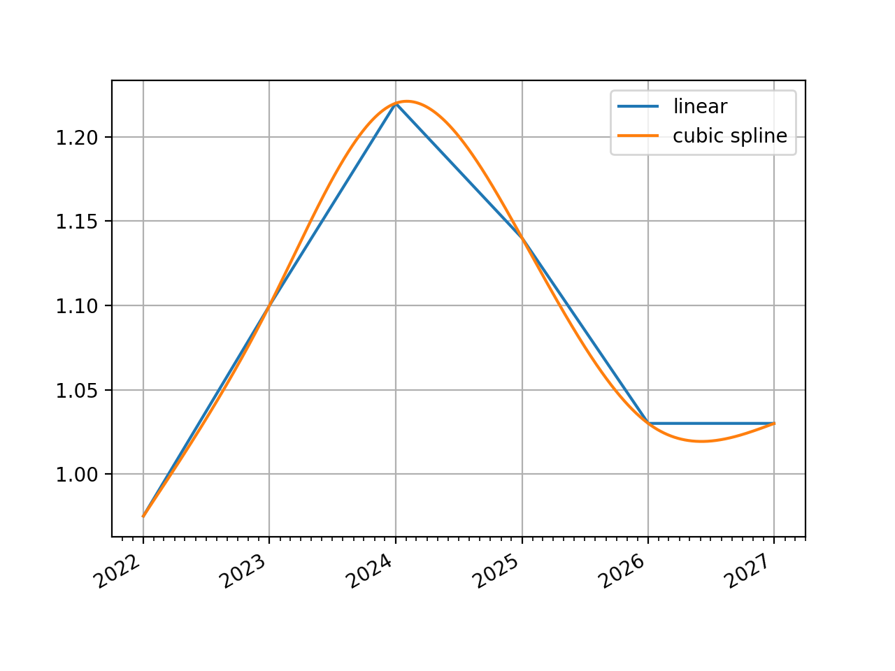
In [1]: nodes = {
   ...:     dt(2022,1,1): 0.975,  # <- initial value is general
   ...:     dt(2023,1,1): 1.10,
   ...:     dt(2024,1,1): 1.22,
   ...:     dt(2025,1,1): 1.14,
   ...:     dt(2026,1,1): 1.03,
   ...:     dt(2027,1,1): 1.03,
   ...: }
   ...:

In [2]: line_curve1 = LineCurve(nodes=nodes, interpolation="linear")

In [3]: line_curve2 = LineCurve(nodes=nodes, interpolation="spline")

In [4]: line_curve1.plot("1d", comparators=[line_curve2], labels=["linear", "cubic spline"])
Out[4]:
(<Figure size 640x480 with 1 Axes>,
 <Axes: >,
 [<matplotlib.lines.Line2D at 0x11283ba10>,
  <matplotlib.lines.Line2D at 0x11283b8c0>])
(
Source code,png,hires.png,pdf)
Attributes Summary
Int in {0,1,2} describing the AD order associated with the Curve.
A str identifier to name the Curve used in
Solvermappings.An instance of
_CurveInterpolator.An instance of
_CurveMeta.An instance of
_CurveNodes.Methods Summary
copy()Create an identical copy of the curve object.
csolve()Solves and sets the coefficients,
c, of thePPSpline.index_value(index_date, index_lag[, ...])Calculate the accrued value of the index from the
index_base.plot(tenor[, right, left, comparators, ...])Plot given forward tenor rates from the curve.
plot_index([right, left, comparators, ...])Plot given index values on a Curve.
rate(effective[, termination, modifier, ...])Calculate the rate on the Curve using DFs.
roll(tenor[, id])Create a
RolledCurve: translating the rate space of Self in time.shift(spread[, id])Create a
ShiftedCurve: moving Self vertically in rate space.to_json()Serialize this object to JSON format.
translate(start[, id])Create a
TranslatedCurve: maintaining an identical rate space, but moving the initial node date forwards in time.update([nodes])Update a curves nodes with new, manually input values.
update_meta(key, value)Update a single meta value on the Curve.
update_node(key, value)Update a single node value on the Curve.
Attributes Documentation
- ad#
Int in {0,1,2} describing the AD order associated with the Curve.
- interpolator#
An instance of
_CurveInterpolator.
- meta#
An instance of
_CurveMeta.
- nodes#
An instance of
_CurveNodes.
Methods Documentation
- copy()#
Create an identical copy of the curve object.
- Return type:
Self
- csolve()#
Solves and sets the coefficients,
c, of thePPSpline.- Return type:
None
Notes
Only impacts curves which have a knot sequence,
t, and aPPSpline. Only solves ifcnot given at curve initialisation.Uses the
spline_endpointsattribute on the class to determine the solving method.
- index_value(index_date, index_lag, index_method=IndexMethod.Curve)#
Calculate the accrued value of the index from the
index_base.This method will raise if performed on a ‘values’ type Curve.
- Parameters:
index_date (datetime) – The reference date for which the index value will be returned.
index_lag (int) – The number of months by which to lag the index when determining the value.
index_method (IndexMethod or str in {"curve", "monthly", "daily"}) – The interpolation method for returning the index value. Monthly returns the index value for the start of the month and daily returns a value based on the interpolation between nodes (which is recommended “linear_index) for
InflationCurve.
- Return type:
Notes
The interpolation methods function as follows:
“curve”: will raise if the requested
index_lagdoes not match the lag attributed to the Curve. In the case theindex_lagmatches, then the index value for any date is derived via the implied interpolation for the discount factors of the Curve.\[I_v(m) = \frac{I_b}{v(m)}\]“monthly”: For any date, m, uses the “curve” method having adjusted m in two ways. Firstly it deducts a number of months equal to \(L - L_c\), where L is the given
index_lagand \(L_c\) is the index lag of the Curve. And the day of the month is set to 1.\[\begin{split}&I^{monthly}_v(m) = I_v(m_adj) \\ &\text{where,} \\ &m_adj = Date(Year(m), Month(m) - L + L_c, 1) \\\end{split}\]“daily”: For any date, m, with a given
index_lagperforms calendar day interpolation on surrounding “monthly” values.\[\begin{split}&I^{daily}_v(m) = I^{monthly}_v(m) + \frac{Day(m) - 1}{n} \left ( I^{monthly}_v(m_+) - I^{monthly}_v(m) \right ) \\ &\text{where,} \\ &m_+ = \text{Any date in the month following, }m &n = \text{Calendar days in, } Month(m)\end{split}\]
Examples
The SWESTR rate, for reference value date 6th Sep 2021, was published as 2.375% and the RFR index for that date was 100.73350964. Below we calculate the value that was published for the RFR index on 7th Sep 2021 by the Riksbank.
In [5]: index_curve = Curve(
   ...:     nodes={
   ...:         dt(2021, 9, 6): 1.0,
   ...:         dt(2021, 9, 7): 1 / (1 + 2.375/36000)
   ...:     },
   ...:     index_base=100.73350964,
   ...:     convention="Act360",
   ...:     index_lag=0,
   ...: )
   ...:

In [6]: index_curve.rate(dt(2021, 9, 6), "1d")
Out[6]: 2.3750000000015703

In [7]: index_curve.index_value(dt(2021, 9, 7), 0)
Out[7]: 100.7401552534832
- plot(tenor, right=NoInput.blank, left=NoInput.blank, comparators=NoInput.blank, difference=False, labels=NoInput.blank)#
Plot given forward tenor rates from the curve. See notes.
- Parameters:
tenor (str) – The tenor of the forward rates to plot, e.g. “1D”, “3M”.
right (datetime or str, optional) – The right bound of the graph. If given as str should be a tenor format defining a point measured from the initial node date of the curve. Defaults to the final node of the curve minus the
tenor.left (datetime or str, optional) – The left bound of the graph. If given as str should be a tenor format defining a point measured from the initial node date of the curve. Defaults to the initial node of the curve.
comparators (list[Curve]) – A list of curves which to include on the same plot as comparators.
difference (bool) – Whether to plot as comparator minus base curve or outright curve levels in plot. Default is False.
labels (list[str]) – A list of strings associated with the plot and comparators. Must be same length as number of plots.
- Returns:
(fig, ax, line)
- Return type:
Matplotlib.Figure, Matplotplib.Axes, Matplotlib.Lines2D
Notes
This function plots single-period, simple interest curve rates, which are defined as:
\[1 + r d = \frac{v_{start}}{v_{end}}\]where d is the day count fraction determined using the
conventionassociated with the Curve.This function does not plot swap rates, which is impossible since the Curve object contains no information regarding the parameters of the ‘swap’ (e.g. its frequency or its convention etc.). If
tenorslonger than one year are sought results may start to deviate from those one might expect. See Issue 246.
- plot_index(right=NoInput.blank, left=NoInput.blank, comparators=NoInput.blank, difference=False, labels=NoInput.blank, interpolation='curve')#
Plot given index values on a Curve.
- Parameters:
right (datetime or str, optional) – The right bound of the graph. If given as str should be a tenor format defining a point measured from the initial node date of the curve. Defaults to the final node of the curve minus the
tenor.left (datetime or str, optional) – The left bound of the graph. If given as str should be a tenor format defining a point measured from the initial node date of the curve. Defaults to the initial node of the curve.
comparators (list[Curve]) – A list of curves which to include on the same plot as comparators.
difference (bool) – Whether to plot as comparator minus base curve or outright curve levels in plot. Default is False.
labels (list[str]) – A list of strings associated with the plot and comparators. Must be same length as number of plots.
interpolation (str in {"curve", "daily", "monthly"}) – The type of index interpolation method to use.
- Returns:
(fig, ax, line)
- Return type:
Matplotlib.Figure, Matplotplib.Axes, Matplotlib.Lines2D
- rate(effective, termination=NoInput.blank, modifier=NoInput.inherit, float_spread=NoInput.blank, spread_compound_method=NoInput.blank)#
Calculate the rate on the Curve using DFs.
If rates are sought for dates prior to the initial node of the curve None will be returned.
- Parameters:
effective (datetime) – The start date of the period for which to calculate the rate.
termination (datetime or str) – The end date of the period for which to calculate the rate.
modifier (str, optional) – The day rule if determining the termination from tenor. If False is determined from the Curve modifier.
float_spread (float, optional) – A float spread can be added to the rate in certain cases.
spread_compound_method (str in {"none_simple", "isda_compounding"}) – The method if adding a float spread. If “none_simple” is used this results in an exact calculation. If “isda_compounding” or “isda_flat_compounding” is used this results in an approximation.
- Return type:
Notes
Calculating rates from a curve implies that the conventions attached to the specific index, e.g. USD SOFR, or GBP SONIA, are applicable and these should be set at initialisation of the
Curve. Thus, the convention used to calculate therateis taken from theCurvefrom whichrateis called.modifieris only used if a tenor is given as the termination.Major indexes, such as legacy IBORs, and modern RFRs typically use a
conventionwhich is either “Act365F” or “Act360”. These conventions do not need additional parameters, such as the termination of a leg, the frequency or a leg or whether it is a stub to calculate a DCF.Adding Floating Spreads
An optimised method for adding floating spreads to a curve rate is provided. This is quite restrictive and mainly used internally to facilitate other parts of the library.
When
spread_compound_methodis “none_simple” the spread is a simple linear addition.When using “isda_compounding” or “isda_flat_compounding” the curve is assumed to be comprised of RFR rates and an approximation is used to derive to total rate.
Examples
In [8]: curve_act365f = Curve(
   ...:     nodes={
   ...:         dt(2022, 1, 1): 1.0,
   ...:         dt(2022, 2, 1): 0.98,
   ...:         dt(2022, 3, 1): 0.978,
   ...:     },
   ...:     convention='Act365F'
   ...: )
   ...:

In [9]: curve_act365f.rate(dt(2022, 2, 1), dt(2022, 3, 1))
Out[9]: 2.6657902424774402
Using a different convention will result in a different rate:
In [10]: curve_act360 = Curve(
   ....:     nodes={
   ....:         dt(2022, 1, 1): 1.0,
   ....:         dt(2022, 2, 1): 0.98,
   ....:         dt(2022, 3, 1): 0.978,
   ....:     },
   ....:     convention='Act360'
   ....: )
   ....:

In [11]: curve_act360.rate(dt(2022, 2, 1), dt(2022, 3, 1))
Out[11]: 2.6292725679229547
- roll(tenor, id=NoInput.blank)#
Create a
RolledCurve: translating the rate space of Self in time.For examples see the documentation for
RolledCurve.- Parameters:
tenor (datetime, str or int) – The measure of time by which to translate the curve through time.
id (str, optional) – Set the id of the returned curve.
- Return type:
- shift(spread, id=NoInput.blank)#
Create a
ShiftedCurve: moving Self vertically in rate space.For examples see the documentation for
ShiftedCurve.- Parameters:
- Return type:
- to_json()#
Serialize this object to JSON format.
The object can be deserialized using the
from_json()method.- Return type:
str
Notes
Some Curves will not be serializable, for example those that possess user defined interpolation functions.
- translate(start, id=NoInput.blank)#
Create a
TranslatedCurve: maintaining an identical rate space, but moving the initial node date forwards in time.For examples see the documentation for
TranslatedCurve.- Parameters:
start (datetime) – The new initial node date for the curve. Must be after the original initial node date.
id (str, optional) – Set the id of the returned curve.
- Return type:
- update(nodes=NoInput.blank)#
Update a curves nodes with new, manually input values.
For arguments see
Curve. Any value not given will not change the underlying Curve.- Parameters:
nodes (dict[datetime, DualTypes], optional) – New nodes to assign to the curve.
- Return type:
None
Notes
Warning
Rateslib is an object-oriented library that uses complex associations. Although Python may not object to directly mutating attributes of a Curve instance, this should be avoided in rateslib. Only use official
updatemethods to mutate the values of an existing Curve instance. This class is labelled as a mutable on update object.
- update_meta(key, value)#
Update a single meta value on the Curve.
- Parameters:
key (datetime) – The meta descriptor to update. Must be a documented attribute of
_CurveMeta.value (Any) – Value to update on the Curve.
- Return type:
None
- update_node(key, value)#
Update a single node value on the Curve.
- Parameters:
- Return type:
None
Notes
Warning
Rateslib is an object-oriented library that uses complex associations. Although Python may not object to directly mutating attributes of a Curve instance, this should be avoided in rateslib. Only use official
updatemethods to mutate the values of an existing Curve instance. This class is labelled as a mutable on update object.