
Curves#
The rateslib.curves module allows flexible curve objects to be created, which
can then, also, be calibrated by a Solver and market instruments.
Rateslib makes a distinction between two fundamentally different
_CurveType. One is values based and one is discount factor (DF)
based.
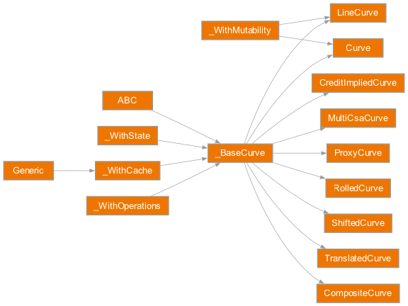
The fundamental object is the _BaseCurve abstract base class (which
provides a generic object to allow users to implement their own custom Curve). All
curve types in rateslib inherit this class and provide its methods and operations. All that is
required for an object to inherit a _BaseCurve is that it provides
a __getitem__() method.
The methods available to any _BaseCurve, based on its
specified binary _CurveType classification are described below:
Operation |
_CurveType.values |
_CurveType.dfs |
|---|---|---|
__getitem__(date) |
Must return rates. |
Must return DFs (or survival probabilities implying hazard rates). |
Returns just the rate associated with |
Returns rates with more features; can imply rates of different tenors or add |
|
Creates a (date, rate) plot. |
Creates a (date, rate) plot with the additional features as above. |
|
Add a |
Add a |
|
Translate the rate space in time. |
Translate the rate space in time. |
|
Translate only the initial node date forward in time. |
Translate only the initial node date forward in time. |
|
Not available. |
Returns index values provided the |
|
Not available. |
Creates a (date, index_value) plot provided the above requirements. |
The two main user curve classes are listed below:
|
A |
|
A |
Introduction#
To create a simple curve, with localised interpolation, minimal configuration is
required, only the nodes are required.
In [1]: from rateslib import dt

In [2]: curve = Curve(
   ...:     nodes={
   ...:         dt(2022,1,1): 1.0,  # <- initial DF (/survival probability) should always be 1.0
   ...:         dt(2023,1,1): 0.99,
   ...:         dt(2024,1,1): 0.979,
   ...:         dt(2025,1,1): 0.967,
   ...:         dt(2026,1,1): 0.956,
   ...:         dt(2027,1,1): 0.946,
   ...:     },
   ...:     interpolation="log_linear",
   ...: )
   ...:
We can also use a similar configuration for a generalised curve constructed from connecting lines between values.
In [3]: linecurve = LineCurve(
   ...:     nodes={
   ...:         dt(2022,1,1): 0.975,  # <- initial value is general
   ...:         dt(2023,1,1): 1.10,
   ...:         dt(2024,1,1): 1.22,
   ...:         dt(2025,1,1): 1.14,
   ...:         dt(2026,1,1): 1.03,
   ...:         dt(2027,1,1): 1.03,
   ...:     },
   ...:     interpolation="linear",
   ...: )
   ...:
Initial Node Date#
The initial node date for either curve type is important because it is implied
to be the date of the construction of the curve (i.e. today’s date).
When a Curve acts as a discount curve any net present
values (NPVs) might assume other features
from this initial node, e.g. the regular settlement date of securities.
This is the also the reason the initial discount factor should also
be exactly 1.0 on a Curve.
The only exception to this is when building a curve used to forecast values, such as index values and inflation prints, it may be practical to start the curve using the most recent inflation print which is usually assigned to the start of the month, thus this may be before today.
Get Item#
As mentioned, any _BaseCurve type has a
__getitem__() method appropriate to its
_CurveType.
Note
DFs (and values) before the curve’s initial node date return zero, in order to value historical cashflows at zero.
Warning
DFs and values after the curve’s final node date will return a value that is an extrapolation. This may not be a sensible or well constrained value depending upon the interpolation method.
In [4]: curve[dt(2022, 9, 26)]
Out[4]: 0.9926477364206718

In [5]: curve[dt(1999, 12, 31)]  # <- before the curve initial node date
Out[5]: 0.0

In [6]: curve[dt(2032, 1, 1)]  # <- extrapolated after the curve final node date
Out[6]: 0.8975214680350941
In [7]: linecurve[dt(2022, 9, 26)]
Out[7]: 1.0667808219178083

In [8]: linecurve[dt(1999, 12, 31)]  # <- before the curve initial node date
Out[8]: 0.0

In [9]: linecurve[dt(2032, 1, 1)]  # <- extrapolated after the curve final node date
Out[9]: 1.03
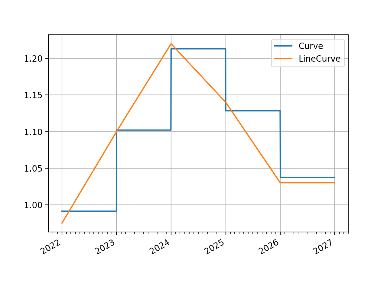
Visualization#
Visualization methods, of rates, are also available via
_BaseCurve.plot(). This allows the easy
inspection of curves directly. Below we demonstrate a plot highlighting the
differences between our parametrised Curve
and LineCurve.
In [10]: curve.plot(
   ....:     "1D",
   ....:     comparators=[linecurve],
   ....:     labels=["Curve", "LineCurve"]
   ....: )
   ....:
Out[10]:
(<Figure size 640x480 with 1 Axes>,
 <Axes: >,
 [<matplotlib.lines.Line2D at 0x13bb7e900>,
  <matplotlib.lines.Line2D at 0x13bb7ea50>])
(Source code, png, hires.png, pdf)
Interpolation#
Rateslib treats curve interpolation in two ways;
it allows a
_CurveSplinewith defined knot sequence for interpolatingnodeswith a cubicPPSpline.it allows local interpolation which uses some function to derive a result from only the immediately neighbouring
nodesto the input date.
If a spline is specified and date falls between its knots it will take precedence. Otherwise, if the date falls outside of the knots or if a spline is not specified then local interpolation functions are used.
The available local interpolation options are described in the documentation for each curve class, and also in supplementary materials, generally they allow the commonly used “linear”, “log_linear”, “flat_forward” varieties as well as others.
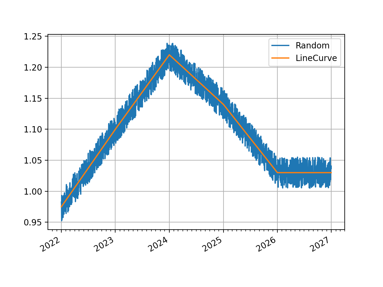
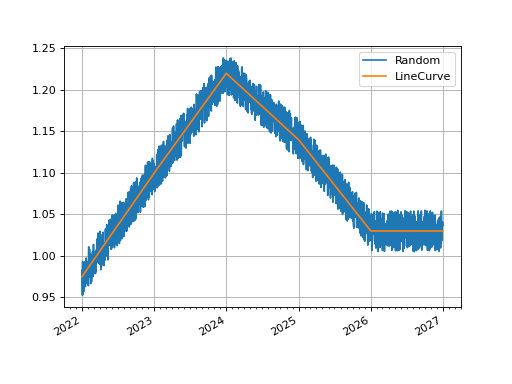
interpolation can also be specified as a user defined function, which allows more
flexibility than just local interpolation if required. See
class documentation for required argument signature.
In [11]: def linear_with_randomness(date, curve):
   ....:     from rateslib.curves.interpolation import index_left
   ....:     from random import random
   ....:     i = index_left(curve.nodes.keys, curve.nodes.n, date)
   ....:     x_1, x_2 = curve.nodes.keys[i], curve.nodes.keys[i + 1]
   ....:     y_1, y_2 = curve.nodes.values[i], curve.nodes.values[i + 1]
   ....:     return (random() -0.5) * 0.05 + y_1 + (y_2 - y_1) * (date - x_1) / (x_2 - x_1)
   ....:

In [12]: random_lc = LineCurve(
   ....:     nodes={
   ....:         dt(2022,1,1): 0.975,  # <- initial value is general
   ....:         dt(2023,1,1): 1.10,
   ....:         dt(2024,1,1): 1.22,
   ....:         dt(2025,1,1): 1.14,
   ....:         dt(2026,1,1): 1.03,
   ....:         dt(2027,1,1): 1.03,
   ....:     },
   ....:     interpolation=linear_with_randomness,
   ....: )
   ....:

In [13]: random_lc.plot("1D", comparators=[linecurve], labels=["Random", "LineCurve"])
Out[13]:
(<Figure size 640x480 with 1 Axes>,
 <Axes: >,
 [<matplotlib.lines.Line2D at 0x13ce74050>,
  <matplotlib.lines.Line2D at 0x13ce741a0>])
(Source code, png, hires.png, pdf)
Spline Interpolation#
Splines can be automatically created by adding interpolation="spline" to the initialization
of a curve. This will define a default knot sequence that encompasses the whole of the
nodes domain. DF based curves’ splines will interpolate over the logarithm of DFs, whilst
values based curves’ splines interpolate directly over those values.
Greater customisation is achieved by directly supplying the knot sequence as the t
argument to a curve initialization. This is a list of datetimes and follows the
appropriate mathematical convention for such sequences (see pp splines).
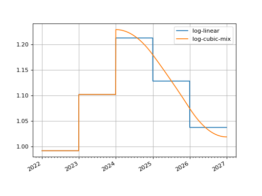
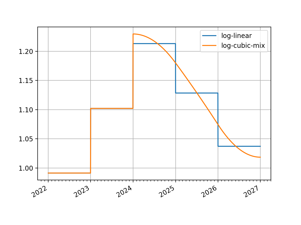
Mixed Interpolation#
Prior to the initial knot in the sequence the local interpolation method is used. This allows curves to be constructed with a mixed interpolation in two parts of the curve. This is common practice for interest rate curves usually with a log-linear short end and a log-cubic spline longer end.
In [14]: mixed_curve = Curve(
   ....:     nodes={
   ....:         dt(2022,1,1): 1.0,
   ....:         dt(2023,1,1): 0.99,
   ....:         dt(2024,1,1): 0.979,
   ....:         dt(2025,1,1): 0.967,
   ....:         dt(2026,1,1): 0.956,
   ....:         dt(2027,1,1): 0.946,
   ....:     },
   ....:     interpolation="log_linear",
   ....:     t = [dt(2024,1,1), dt(2024,1,1), dt(2024,1,1), dt(2024,1,1),
   ....:          dt(2025,1,1),
   ....:          dt(2026,1,1),
   ....:          dt(2027,1,1), dt(2027,1,1), dt(2027,1,1), dt(2027,1,1)]
   ....: )
   ....:

In [15]: curve.plot("1D", comparators=[mixed_curve], labels=["log-linear", "log-cubic-mix"])
Out[15]:
(<Figure size 640x480 with 1 Axes>,
 <Axes: >,
 [<matplotlib.lines.Line2D at 0x13cda16a0>,
  <matplotlib.lines.Line2D at 0x13cda17f0>])
(Source code, png, hires.png, pdf)

IBOR or RFR#
The different Instruments in rateslib may require
different interest rate index types, be it IBOR or RFR based. These are
fundamentally different and require care dependent on
which curve type: Curve or
LineCurve is used.
Curve Type |
RFR Based |
IBOR Based |
|---|---|---|
DFs are value date based. For an RFR rate applicable between a start and end date, the start and end date DFs will reflect this rate, regardless of the publication timeframe of the rate. |
DFs are value date based. For an IBOR rate applicable between a start and end date, the start and end date DFs will reflect this rate, regardless of the publication timeframe of the rate. |
|
Rates are labelled by reference value date, not publication date. |
Rates are labelled by publication date, not reference value date. |
Since DF based curves behave similarly for each index type we will give an example
of constructing an IRS under the different methods.
For an RFR curve the nodes values are by reference date. The 3.0% value which
is applicable between the reference date of 2nd Jan ‘22 and end date 3rd Jan ‘22,
is indexed according to the 2nd Jan ‘22.
In [16]: rfr_curve = LineCurve(
   ....:     nodes={
   ....:         dt(2022, 1, 1): 2.0,
   ....:         dt(2022, 1, 2): 3.0,
   ....:         dt(2022, 1, 3): 4.0
   ....:     }
   ....: )
   ....:

In [17]: p = FloatPeriod(
   ....:     start=dt(2022, 2, 1),
   ....:     end=dt(2022, 2, 2),
   ....:     payment=dt(2022, 2, 2),
   ....:     frequency="1B",
   ....:     convention="Act360",
   ....:     fixing_series="usd_rfr"
   ....: )
   ....:

In [18]: p.rate(rate_curve=rfr_curve)
Out[18]: np.float64(33.00000000000036)
For an IBOR curve the nodes values are by publication date. The curve below has a
lag of 2 business days. and the publication on 1st Jan ‘22 is applicable to the
reference value date of 3rd Jan.
In [19]: ibor_curve = LineCurve(
   ....:     nodes={
   ....:         dt(2022, 1, 1): 2.5,
   ....:         dt(2022, 1, 2): 3.5,
   ....:         dt(2022, 1, 3): 4.5
   ....:     }
   ....: )
   ....:

In [20]: p = FloatPeriod(
   ....:     start=dt(2022, 2, 3),
   ....:     end=dt(2022, 3, 3),
   ....:     payment=dt(2022, 3, 3),
   ....:     frequency="1M",
   ....:     convention="Act360",
   ....:     fixing_series="usd_ibor"
   ....: )
   ....:

In [21]: p.rate(rate_curve=ibor_curve)
Out[21]: np.float64(49.318706334755)
Mutable Pricing Objects#
The only curves with parameters that are mutated and solved by a Solver
are Curve and LineCurve. These are
classed as Pricing Objects.
These curves inherit the _WithMutability mixin.
Pricing Containers#
Other objects that are available, that are constructed via manipulations of the base Pricing Objects (or other Pricing Containers) are the so called Pricing Containers.
The main user curve classes are listed below:
|
A dynamic composition of a sequence of other |
|
A dynamic composition of a sequence of other |
Imply a |
|
|
A |
These objects allow complex curve features and scenarios to be modelled in a recognisable and easily parametrised format.
The following Pricing Containers are also created as the result of certain operations, which any
_BaseCurve can inherit using the _WithOperations
mixin.
|
Create a new |
|
Create a new |
|
Create a new |