A EURUSD market for IRS, cross-currency and FX volatility#

In this notebook we demonstrate the code for rateslib to build:

local currency interest rate curves in EUR and USD from RFR swaps,
collateral curves accounting for the cross-currency basis and FX swap points,
volatility surface priced from FX volatility products.

Input market data#

First things first we need market data for the interest rates curves and forward FX curves. This data was observed on 28th May 2024.

[1]:

from rateslib import *
import numpy as np
from pandas import DataFrame

[2]:

fxr = FXRates({"eurusd": 1.0867}, settlement=dt(2024, 5, 30))

[3]:

mkt_data = DataFrame(
    data=[['1w', 3.9035,5.3267,3.33,],
          ['2w', 3.9046,5.3257,6.37,],
          ['3w',3.8271,5.3232,9.83,],
          ['1m',3.7817,5.3191,13.78,],
          ['2m',3.7204,5.3232,30.04,],
          ['3m',3.667,5.3185,45.85,-2.5],
          ['4m',3.6252,5.3307,61.95,],
          ['5m',3.587,5.3098,78.1,],
          ['6m',3.5803,5.3109,94.25,-3.125],
          ['7m',3.5626,5.301,110.82,],
          ['8m',3.531,5.2768,130.45,],
          ['9m',3.5089,5.2614,145.6,-7.25],
          ['10m',3.4842,5.2412,162.05,],
          ['11m',3.4563,5.2144,178,],
          ['1y',3.4336,5.1936,None,-6.75],
          ['15m',3.3412,5.0729,None,-6.75],
          ['18m',3.2606,4.9694,None,-6.75],
          ['21m',3.1897,4.8797,None,-7.75],
          ['2y',3.1283,4.8022,None,-7.875],
          ['3y',2.9254,4.535,None,-9],
          ['4y',2.81,4.364,None,-10.125],
          ['5y',2.7252,4.256,None,-11.125],
          ['6y',2.6773,4.192,None,-12.125],
          ['7y',2.6541,4.151,None,-13],
          ['8y',2.6431,4.122,None,-13.625],
          ['9y',2.6466,4.103,None,-14.25],
          ['10y',2.6562,4.091,None,-14.875],
          ['12y',2.6835,4.084,None,-16.125],
          ['15y',2.7197,4.08,None,-17],
          ['20y',2.6849,4.04,None,-16],
          ['25y',2.6032,3.946,None,-12.75],
          ['30y',2.5217,3.847,None,-9.5]],
    columns=["tenor", "estr", "sofr", "fx_swap", "xccy"],
)
mkt_data

[3]:

	tenor	estr	sofr	fx_swap	xccy
0	1w	3.9035	5.3267	3.33	NaN
1	2w	3.9046	5.3257	6.37	NaN
2	3w	3.8271	5.3232	9.83	NaN
3	1m	3.7817	5.3191	13.78	NaN
4	2m	3.7204	5.3232	30.04	NaN
5	3m	3.6670	5.3185	45.85	-2.500
6	4m	3.6252	5.3307	61.95	NaN
7	5m	3.5870	5.3098	78.10	NaN
8	6m	3.5803	5.3109	94.25	-3.125
9	7m	3.5626	5.3010	110.82	NaN
10	8m	3.5310	5.2768	130.45	NaN
11	9m	3.5089	5.2614	145.60	-7.250
12	10m	3.4842	5.2412	162.05	NaN
13	11m	3.4563	5.2144	178.00	NaN
14	1y	3.4336	5.1936	NaN	-6.750
15	15m	3.3412	5.0729	NaN	-6.750
16	18m	3.2606	4.9694	NaN	-6.750
17	21m	3.1897	4.8797	NaN	-7.750
18	2y	3.1283	4.8022	NaN	-7.875
19	3y	2.9254	4.5350	NaN	-9.000
20	4y	2.8100	4.3640	NaN	-10.125
21	5y	2.7252	4.2560	NaN	-11.125
22	6y	2.6773	4.1920	NaN	-12.125
23	7y	2.6541	4.1510	NaN	-13.000
24	8y	2.6431	4.1220	NaN	-13.625
25	9y	2.6466	4.1030	NaN	-14.250
26	10y	2.6562	4.0910	NaN	-14.875
27	12y	2.6835	4.0840	NaN	-16.125
28	15y	2.7197	4.0800	NaN	-17.000
29	20y	2.6849	4.0400	NaN	-16.000
30	25y	2.6032	3.9460	NaN	-12.750
31	30y	2.5217	3.8470	NaN	-9.500

Solving rates curves and FX forwards curve#

We will create all Curves and solve them all using the Solver. It is possible to solve everything simultaneously in a single Solver but this is less efficient than decoupling the known separable components, and using multiple Solvers in a dependency chain.

[4]:

eur = Curve(
    nodes={
        dt(2024, 5, 28): 1.0,
        **{add_tenor(dt(2024, 5, 30), _, "F", "tgt"): 1.0 for _ in mkt_data["tenor"]}
    },
    calendar="tgt",
    interpolation="log_linear",
    convention="act360",
    id="estr",
)
usd = Curve(
    nodes={
        dt(2024, 5, 28): 1.0,
        **{add_tenor(dt(2024, 5, 30), _, "F", "nyc"): 1.0 for _ in mkt_data["tenor"]}
    },
    calendar="nyc",
    interpolation="log_linear",
    convention="act360",
    id="sofr",
)
eurusd = Curve(
    nodes={
        dt(2024, 5, 28): 1.0,
        **{add_tenor(dt(2024, 5, 30), _, "F", "tgt"): 1.0 for _ in mkt_data["tenor"]}
    },
    interpolation="log_linear",
    convention="act360",
    id="eurusd",
)

With Curves created but not necessarily calibrated we can design the FXForwards market mapping:

[5]:

fxf = FXForwards(
    fx_rates=fxr,
    fx_curves={"eureur": eur, "eurusd": eurusd, "usdusd": usd}
)

The Instruments used to solve the ESTR curve are ESTR swaps and the SOFR curve are SOFR swaps:

[6]:

estr_swaps = [IRS(dt(2024, 5, 30), _, spec="eur_irs", curves="estr") for _ in mkt_data["tenor"]]
estr_rates = mkt_data["estr"].tolist()
labels = mkt_data["tenor"].to_list()
sofr_swaps =  [IRS(dt(2024, 5, 30), _, spec="usd_irs", curves="sofr") for _ in mkt_data["tenor"]]
sofr_rates = mkt_data["sofr"].tolist()

[7]:

eur_solver = Solver(
    curves=[eur],
    instruments=estr_swaps,
    s=estr_rates,
    fx=fxf,
    instrument_labels=labels,
    id="eur",
)
usd_solver = Solver(
    curves=[usd],
    instruments=sofr_swaps,
    s=sofr_rates,
    fx=fxf,
    instrument_labels=labels,
    id="usd",
)

SUCCESS: `func_tol` reached after 7 iterations (levenberg_marquardt), `f_val`: 1.6125193512590306e-15, `time`: 0.1638s
SUCCESS: `func_tol` reached after 7 iterations (levenberg_marquardt), `f_val`: 3.993406376879668e-17, `time`: 0.1608s

The cross currency curve use a combination of FXSwaps and XCS:

[8]:

fxswaps = [FXSwap(dt(2024, 5, 30), _, pair="eurusd", curves=[None, "eurusd", None, "sofr"]) for _ in mkt_data["tenor"][0:14]]
fxswap_rates = mkt_data["fx_swap"][0:14].tolist()
xcs = [XCS(dt(2024, 5, 30), _, spec="eurusd_xcs", curves=["estr", "eurusd", "sofr", "sofr"]) for _ in mkt_data["tenor"][14:]]
xcs_rates = mkt_data["xccy"][14:].tolist()

[9]:

fx_solver = Solver(
    pre_solvers=[eur_solver, usd_solver],
    curves=[eurusd],
    instruments=fxswaps + xcs,
    s=fxswap_rates + xcs_rates,
    fx=fxf,
    instrument_labels=labels,
    id="eurusd_xccy",
)

SUCCESS: `func_tol` reached after 5 iterations (levenberg_marquardt), `f_val`: 2.732818069605529e-21, `time`: 1.0999s

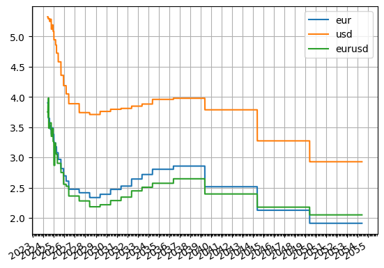
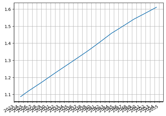
Solved Interest Rate Curves and FX Forward Rates#

OK so thats all the interest rates curves solved and the FX forwards rates are all available now. Do a quick plot just for interest:

[10]:

eur.plot("1d", comparators=[usd, eurusd], labels=["eur", "usd", "eurusd"])

[10]:

(<Figure size 640x480 with 1 Axes>,
 <Axes: >,
 [<matplotlib.lines.Line2D at 0x10d3a9f90>,
  <matplotlib.lines.Line2D at 0x10e19ee90>,
  <matplotlib.lines.Line2D at 0x10e19ec10>])

[11]:

fxf.plot("eurusd")

[11]:

(<Figure size 640x480 with 1 Axes>,
 <Axes: >,
 [<matplotlib.lines.Line2D at 0x10ea3f750>])

Solving an FX Vol Surface#

Next we will use the market FX volatility quotes to build a surface. These prices are all expressed in log-normal vol terms under normal market conventions and the instruments 1Y or less use spot unadjusted delta and those longer than 1y use forward undajusted delta.

[12]:

vol_data = DataFrame(
    data=[
        ['1w',4.535,-0.047,0.07,-0.097,0.252],
        ['2w',5.168,-0.082,0.077,-0.165,0.24],
        ['3w',5.127,-0.175,0.07,-0.26,0.233],
        ['1m',5.195,-0.2,0.07,-0.295,0.235],
        ['2m',5.237,-0.28,0.087,-0.535,0.295],
        ['3m',5.257,-0.363,0.1,-0.705,0.35],
        ['4m',5.598,-0.47,0.123,-0.915,0.422],
        ['5m',5.776,-0.528,0.133,-1.032,0.463],
        ['6m',5.92,-0.565,0.14,-1.11,0.49],
        ['9m',6.01,-0.713,0.182,-1.405,0.645],
        ['1y',6.155,-0.808,0.23,-1.585,0.795],
        ['18m',6.408,-0.812,0.248,-1.588,0.868],
        ['2y',6.525,-0.808,0.257,-1.58,0.9],
        ['3y',6.718,-0.733,0.265,-1.45,0.89],
        ['4y',7.025,-0.665,0.265,-1.31,0.885],
        ['5y',7.26,-0.62,0.26,-1.225,0.89],
        ['6y',7.508,-0.516,0.27,-0.989,0.94],
        ['7y',7.68,-0.442,0.278,-0.815,0.975],
        ['10y',8.115,-0.267,0.288,-0.51,1.035],
        ['15y',8.652,-0.325,0.362,-0.4,1.195],
        ['20y',8.651,-0.078,0.343,-0.303,1.186],
        ['25y',8.65,-0.029,0.342,-0.218,1.178],
        ['30y',8.65,0.014,0.341,-0.142,1.171],
    ],
    columns=["tenor", "atm", "25drr", "25dbf", "10drr", "10dbf"]
)
vol_data["expiry"] = [add_tenor(dt(2024, 5, 28), _, "MF", "tgt") for _ in vol_data["tenor"]]
vol_data

[12]:

	tenor	atm	25drr	25dbf	10drr	10dbf	expiry
0	1w	4.535	-0.047	0.070	-0.097	0.252	2024-06-04
1	2w	5.168	-0.082	0.077	-0.165	0.240	2024-06-11
2	3w	5.127	-0.175	0.070	-0.260	0.233	2024-06-18
3	1m	5.195	-0.200	0.070	-0.295	0.235	2024-06-28
4	2m	5.237	-0.280	0.087	-0.535	0.295	2024-07-29
5	3m	5.257	-0.363	0.100	-0.705	0.350	2024-08-28
6	4m	5.598	-0.470	0.123	-0.915	0.422	2024-09-30
7	5m	5.776	-0.528	0.133	-1.032	0.463	2024-10-28
8	6m	5.920	-0.565	0.140	-1.110	0.490	2024-11-28
9	9m	6.010	-0.713	0.182	-1.405	0.645	2025-02-28
10	1y	6.155	-0.808	0.230	-1.585	0.795	2025-05-28
11	18m	6.408	-0.812	0.248	-1.588	0.868	2025-11-28
12	2y	6.525	-0.808	0.257	-1.580	0.900	2026-05-28
13	3y	6.718	-0.733	0.265	-1.450	0.890	2027-05-28
14	4y	7.025	-0.665	0.265	-1.310	0.885	2028-05-29
15	5y	7.260	-0.620	0.260	-1.225	0.890	2029-05-28
16	6y	7.508	-0.516	0.270	-0.989	0.940	2030-05-28
17	7y	7.680	-0.442	0.278	-0.815	0.975	2031-05-28
18	10y	8.115	-0.267	0.288	-0.510	1.035	2034-05-29
19	15y	8.652	-0.325	0.362	-0.400	1.195	2039-05-30
20	20y	8.651	-0.078	0.343	-0.303	1.186	2044-05-30
21	25y	8.650	-0.029	0.342	-0.218	1.178	2049-05-28
22	30y	8.650	0.014	0.341	-0.142	1.171	2054-05-28

A Surface is defined by given expiries and delta grdipoints. All vol values are initially set to 5.0, and will be calibrated by the Instruments.

[13]:

surface = FXDeltaVolSurface(
    eval_date=dt(2024, 5, 28),
    expiries=vol_data["expiry"],
    delta_indexes=[0.1, 0.25, 0.5, 0.75, 0.9],
    node_values=np.ones((23, 5))*5.0,
    delta_type="forward",
    id="eurusd_vol"
)

Define the instruments and their rates for 1Y or less:

[14]:

fx_args = dict(
    pair="eurusd",
    curves=[None, "eurusd", None, "sofr"],
    calendar="tgt",
    delivery_lag=2,
    payment_lag=2,
    eval_date=dt(2024, 5, 28),
    modifier="MF",
    premium_ccy="usd",
    vol="eurusd_vol",
)

instruments_le_1y, rates_le_1y, labels_le_1y = [], [], []
for row in range(11):
    instruments_le_1y.extend([
        FXStraddle(strike="atm_delta", expiry=vol_data["expiry"][row], delta_type="spot", **fx_args),
        FXRiskReversal(strike=("-25d", "25d"), expiry=vol_data["expiry"][row], delta_type="spot", **fx_args),
        FXBrokerFly(strike=(("-25d", "25d"), "atm_delta"), expiry=vol_data["expiry"][row], delta_type="spot", **fx_args),
        FXRiskReversal(strike=("-10d", "10d"), expiry=vol_data["expiry"][row], delta_type="spot", **fx_args),
        FXBrokerFly(strike=(("-10d", "10d"), "atm_delta"), expiry=vol_data["expiry"][row], delta_type="spot", **fx_args),
    ])
    rates_le_1y.extend([vol_data["atm"][row], vol_data["25drr"][row], vol_data["25dbf"][row], vol_data["10drr"][row], vol_data["10dbf"][row]])
    labels_le_1y.extend([f"atm_{row}", f"25drr_{row}", f"25dbf_{row}", f"10drr_{row}", f"10dbf_{row}"])

Also define the instruments and rates for greater than 1Y:

[15]:

instruments_gt_1y, rates_gt_1y, labels_gt_1y = [], [], []
for row in range(11, 23):
    instruments_gt_1y.extend([
        FXStraddle(strike="atm_delta", expiry=vol_data["expiry"][row], delta_type="forward", **fx_args),
        FXRiskReversal(strike=("-25d", "25d"), expiry=vol_data["expiry"][row], delta_type="forward", **fx_args),
        FXBrokerFly(strike=(("-25d", "25d"), "atm_delta"), expiry=vol_data["expiry"][row], delta_type="forward", **fx_args),
        FXRiskReversal(strike=("-10d", "10d"), expiry=vol_data["expiry"][row], delta_type="forward", **fx_args),
        FXBrokerFly(strike=(("-10d", "10d"), "atm_delta"), expiry=vol_data["expiry"][row], delta_type="forward", **fx_args),
    ])
    rates_gt_1y.extend([vol_data["atm"][row], vol_data["25drr"][row], vol_data["25dbf"][row], vol_data["10drr"][row], vol_data["10dbf"][row]])
    labels_gt_1y.extend([f"atm_{row}", f"25drr_{row}", f"25dbf_{row}", f"10drr_{row}", f"10dbf_{row}"])

Now solve for all calibrating instruments and rates.

[16]:

surface_solver = Solver(
    surfaces=[surface],
    instruments=instruments_le_1y+instruments_gt_1y,
    s=rates_le_1y+rates_gt_1y,
    instrument_labels=labels_le_1y+labels_gt_1y,
    fx=fxf,
    pre_solvers=[fx_solver],
    id="eurusd_vol"
)

SUCCESS: `func_tol` reached after 11 iterations (levenberg_marquardt), `f_val`: 1.2685386049514868e-15, `time`: 3.6423s

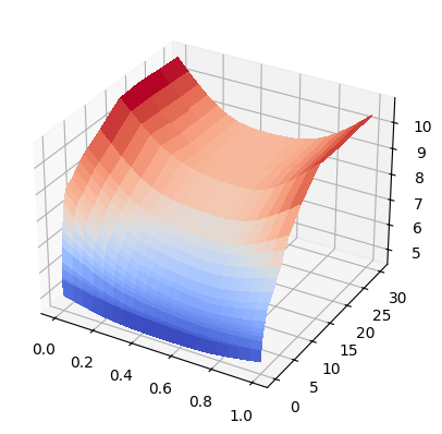
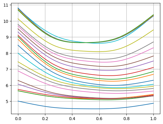
3D Surface Plot and Cross-sectional Smiles#

[17]:

surface.plot()

[17]:

(<Figure size 640x480 with 1 Axes>, <Axes3D: >, None)

[18]:

surface.smiles[0].plot(comparators=surface.smiles[1:])

[18]:

(<Figure size 640x480 with 1 Axes>,
 <Axes: >,
 [<matplotlib.lines.Line2D at 0x10f34d590>,
  <matplotlib.lines.Line2D at 0x10f34d6d0>,
  <matplotlib.lines.Line2D at 0x10f34d810>,
  <matplotlib.lines.Line2D at 0x10f34d950>,
  <matplotlib.lines.Line2D at 0x10f34da90>,
  <matplotlib.lines.Line2D at 0x10f34dbd0>,
  <matplotlib.lines.Line2D at 0x10f34dd10>,
  <matplotlib.lines.Line2D at 0x10f34de50>,
  <matplotlib.lines.Line2D at 0x10f34df90>,
  <matplotlib.lines.Line2D at 0x10f34e0d0>,
  <matplotlib.lines.Line2D at 0x10f34e210>,
  <matplotlib.lines.Line2D at 0x10f34e350>,
  <matplotlib.lines.Line2D at 0x10f34e490>,
  <matplotlib.lines.Line2D at 0x10f34e5d0>,
  <matplotlib.lines.Line2D at 0x10f34e710>,
  <matplotlib.lines.Line2D at 0x10f34e850>,
  <matplotlib.lines.Line2D at 0x10f34e990>,
  <matplotlib.lines.Line2D at 0x10f34ead0>,
  <matplotlib.lines.Line2D at 0x10f34ec10>,
  <matplotlib.lines.Line2D at 0x10f34ed50>,
  <matplotlib.lines.Line2D at 0x10f34ee90>,
  <matplotlib.lines.Line2D at 0x10f34efd0>,
  <matplotlib.lines.Line2D at 0x10f34f110>])

SABR Surface#

It is also possible to create and solve a SABR Surface constructed with SABR Smiles.

[19]:

sabr_surface = FXSabrSurface(
    eval_date=dt(2024, 5, 28),
    expiries=list(vol_data["expiry"]),
    node_values=[[0.05, 1.0, 0.01, 0.10]] * 23,  # alpha, beta, rho, nu
    pair="eurusd",
    delivery_lag=2,
    calendar="tgt|fed",
    id="eurusd_vol",
)
surface_solver = Solver(
    surfaces=[sabr_surface],
    instruments=instruments_le_1y+instruments_gt_1y,
    s=rates_le_1y+rates_gt_1y,
    instrument_labels=labels_le_1y+labels_gt_1y,
    fx=fxf,
    pre_solvers=[fx_solver],
    id="eurusd_vol",
    conv_tol=1e-5,
)

SUCCESS: `conv_tol` reached after 14 iterations (levenberg_marquardt), `f_val`: 0.06105586702869039, `time`: 9.4891s

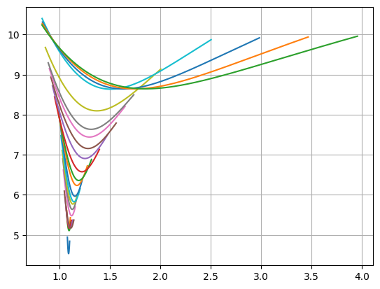
Here the plot is measured relative to strike.

[20]:

sabr_surface.smiles[0].plot(f=fxf, comparators=sabr_surface.smiles[1:])

[20]:

(<Figure size 640x480 with 1 Axes>,
 <Axes: >,
 [<matplotlib.lines.Line2D at 0x10f4b5e50>,
  <matplotlib.lines.Line2D at 0x10f4b5f90>,
  <matplotlib.lines.Line2D at 0x10f4b60d0>,
  <matplotlib.lines.Line2D at 0x10f4b6210>,
  <matplotlib.lines.Line2D at 0x10f4b6350>,
  <matplotlib.lines.Line2D at 0x10f4b6490>,
  <matplotlib.lines.Line2D at 0x10f4b65d0>,
  <matplotlib.lines.Line2D at 0x10f4b6710>,
  <matplotlib.lines.Line2D at 0x10f4b6850>,
  <matplotlib.lines.Line2D at 0x10f4b6990>,
  <matplotlib.lines.Line2D at 0x10f4b6ad0>,
  <matplotlib.lines.Line2D at 0x10f4b6c10>,
  <matplotlib.lines.Line2D at 0x10f4b6d50>,
  <matplotlib.lines.Line2D at 0x10f4b6e90>,
  <matplotlib.lines.Line2D at 0x10f4b6fd0>,
  <matplotlib.lines.Line2D at 0x10f4b7110>,
  <matplotlib.lines.Line2D at 0x10f4b7250>,
  <matplotlib.lines.Line2D at 0x10f4b7390>,
  <matplotlib.lines.Line2D at 0x10f4b74d0>,
  <matplotlib.lines.Line2D at 0x10f4b7610>,
  <matplotlib.lines.Line2D at 0x10f4b7750>,
  <matplotlib.lines.Line2D at 0x10f4b7890>,
  <matplotlib.lines.Line2D at 0x10f4b79d0>])

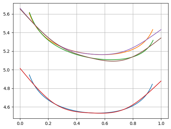
Below the plot is measured versus a forward, unadjusted delta, and also compared with the previous DeltaVolSurface.

Major differences begin to emerge at the extremities, i.e. below 0.1 delta and above 0.9 delta.

[21]:

sabr_surface.smiles[0].plot(f=fxf, comparators=sabr_surface.smiles[1:3]+surface.smiles[0:3], x_axis="delta")

[21]:

(<Figure size 640x480 with 1 Axes>,
 <Axes: >,
 [<matplotlib.lines.Line2D at 0x10f5a9f90>,
  <matplotlib.lines.Line2D at 0x10f5aa0d0>,
  <matplotlib.lines.Line2D at 0x10f5aa210>,
  <matplotlib.lines.Line2D at 0x10f5aa350>,
  <matplotlib.lines.Line2D at 0x10f5aa490>,
  <matplotlib.lines.Line2D at 0x10f5aa5d0>])