Building Custom Curves (Nelson-Siegel)#

The rateslib curves objects are structured in such a way that it is strightforward to create new, custom curve objects useable throughout the library, provided they implement the necessary abstract base objects.

Nelson-Siegel Parametrization#

This example will construct a parametric Nelson-Siegel Curve, whose continuously compounded zero rate, \(r\), at time, \(T\), is given by the following equation of four parameters:

\[\begin{split}r(T) = \begin{bmatrix} \beta_0 & \beta_1 & \beta_2 \end{bmatrix} \begin{bmatrix} 1 \\ \lambda (1- e^{-T/ \lambda}) / T \\ \lambda (1- e^{-T/ \lambda})/ T - e^{-T/ \lambda} \end{bmatrix}\end{split}\]

This leads to the discount factors on that curve equaling:

\[v(T) = e^{-T r(T)}\]

_BaseCurve ABCs#

First we setup the skeletal structure of our custom curve. We will inherit from _BaseCurve and setup the necessary abstract base class (ABC) properties.

Some items we know in advance regarding our custom curve:

it will return discount factors, defining its _CurveType,
it has 4 parameters,
we must define a start date (which makes its initial node) and end in its _CurveNodes
we will just inherit meta property intialisation from the _BaseCurve

[1]:

from rateslib import *
import numpy as np

from rateslib.curves import _BaseCurve, _CurveType, _CurveNodes

class NelsonSiegelCurve(_BaseCurve):

    # ABC properties

    _base_type = _CurveType.dfs
    _id = None
    _meta = None
    _nodes = None
    _ad = None
    _interpolator = None
    _n = 4

    def __init__(self, start, end, beta0, beta1, beta2, lambd):
        self._id = super()._id
        self._meta = super()._meta
        self._ad = 0
        self._nodes = _CurveNodes({start: 0.0, end: 0.0})
        self._params = (beta0, beta1, beta2, lambd)

    # ABC required methods

    def _set_ad_order(self, order):
        raise NotImplementedError()

    def __getitem__(self, date):
        raise NotImplementedError()

This curve can now be initialised without raising any errors relating to Abstract Base Classes. However, it doesn’t do much without implementing the __getitem__ method.

[2]:

curve = NelsonSiegelCurve(dt(2000, 1, 1), dt(2010, 1, 1), 0.025, 0.0, 0.0, 0.5)

The `getitem` method#

This method will return discount factors. If the requested date is prior to the curve: return zero as usual. If the date is the same as the initial node date: return one, else use continuously compounded rates to derive a discount factor.

[3]:

class NelsonSiegelCurve(_BaseCurve):
    _base_type = _CurveType.dfs
    _id = None
    _meta = None
    _nodes = None
    _ad = None
    _interpolator = None
    _n = 4

    def __init__(self, start, end, beta0, beta1, beta2, lambd):
        self._id = super()._id
        self._meta = super()._meta
        self._ad = 0
        self._nodes = _CurveNodes({start: 0.0, end: 0.0})
        self._params = (beta0, beta1, beta2, lambd)

    def _set_ad_order(self, order):
        raise NotImplementedError()

    def __getitem__(self, date):
        if date < self.nodes.initial:
            return 0.0
        elif date == self.nodes.initial:
            return 1.0
        b0, b1, b2, l0 = self._params
        T = dcf(self.nodes.initial, date, convention=self.meta.convention, calendar=self.meta.calendar)
        a1 = l0 * (1 - dual_exp(-T / l0)) / T
        a2 =  a1 - dual_exp(-T / l0)
        r = b0 + a1 * b1 + a2 * b2
        return dual_exp(-T * r)

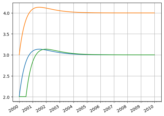
Once this method is added to the class and the discount factors are available, all of the provided methods are also available. The following snippet of code demonstrates each of the rate(), plot(), roll(), shift() and translate() methods without the user having implemented any of them:

[4]:

ns_curve = NelsonSiegelCurve(
    start=dt(2000, 1, 1),
    end=dt(2010, 1, 1),
    beta0=0.03,
    beta1=-0.01,
    beta2=0.01,
    lambd=0.75
)
ns_curve.plot("1b", comparators=[ns_curve.shift(100), ns_curve.roll("6m")])

[4]:

(<Figure size 640x480 with 1 Axes>,
 <Axes: >,
 [<matplotlib.lines.Line2D at 0x110078050>,
  <matplotlib.lines.Line2D at 0x1100a0550>,
  <matplotlib.lines.Line2D at 0x1100a02d0>])

Mutatbility and the `Solver`#

In order to allow this curve to be calibrated by a Solver, we need to add some elements that allows the Solver to interact with it. We will also set the NelsonSeigelCurve to inherit _WithMutability.

Firstly, we can add the getter methods:

[5]:

_ini_solve = 0  #  <-  this tells the `Solver` not to 'skip' any parameters (like the initial DF of 1.0 on a `Curve`)

def _get_node_vector(self):
   # this maps the curve's parameters to a consistent NumPy array consumed by the `Solver`.
   return np.array(self._params)

def _get_node_vars(self):
   # this get the ordered variable names of the curve's parameters for AD management.
   return tuple(f"{self._id}{i}" for i in range(self._ini_solve, self._n))

The setter methods that the Solver needs are slightly more complicated. These allow the Solver to mutate the Curve directly and provide mappings.

[6]:

from rateslib.curves import _WithMutability
from rateslib.mutability import _new_state_post
from rateslib.dual import set_order_convert
from rateslib.dual.utils import _dual_float

@_new_state_post  # <- this sets a new state every time the curve is mutated
def _set_node_vector(self, vector, ad):
    # this maps the `Solver's` output new node values to the curve's parameters attribute with the appropriate AD number type
    if ad == 0:
        self._params = tuple(_dual_float(_) for _ in vector)
    elif ad == 1:
        self._params = tuple(
            Dual(_dual_float(_), [f"{self._id}{i}"], []) for i, _ in enumerate(vector)
        )
    else: # ad == 2
        self._params = tuple(
            Dual2(_dual_float(_), [f"{self._id}{i}"], [], []) for i, _ in enumerate(vector)
        )

def _set_ad_order(self, order):
    # this allows the `Solver` to change the AD number type of the curve for `delta` and `gamma` calculations.
    if self.ad == order:
        return None
    else:
        self._ad = order
        self._params = tuple(
            set_order_convert(_, order, [f"{self._id}{i}"]) for i, _ in enumerate(self._params)
        )

Adding these elements yields the final code to implement this user custom Curve class:

[7]:

class NelsonSiegelCurve(_WithMutability, _BaseCurve):

    # ABC properties

    _ini_solve = 0
    _base_type = _CurveType.dfs
    _id = None
    _meta = None
    _nodes = None
    _ad = None
    _interpolator = None
    _n = 4

    def __init__(self, start, end, beta0, beta1, beta2, lamb):
        self._id = super()._id
        self._meta = super()._meta
        self._ad = 0
        self._nodes = _CurveNodes({start: 0.0, end: 0.0})
        self._params = (beta0, beta1, beta2, lamb)

    def __getitem__(self, date):
        if date < self.nodes.initial:
            return 0.0
        elif date == self.nodes.initial:
            return 1.0
        b0, b1, b2, l0 = self._params
        T = dcf(self.nodes.initial, date, convention=self.meta.convention, calendar=self.meta.calendar)
        a1 = l0 * (1 - dual_exp(-T / l0)) / T
        a2 =  a1 - dual_exp(-T / l0)
        r = b0 + a1 * b1 + a2 * b2
        return dual_exp(-T * r)

    # Solver mutability methods

    def _get_node_vector(self):
        return np.array(self._params)

    def _get_node_vars(self):
        return tuple(f"{self._id}{i}" for i in range(self._ini_solve, self._n))

    def _set_node_vector(self, vector, ad):
        if ad == 0:
            self._params = tuple(_dual_float(_) for _ in vector)
        elif ad == 1:
            self._params = tuple(
                 Dual(_dual_float(_), [f"{self._id}{i}"], []) for i, _ in enumerate(vector)
            )
        else: # ad == 2
            self._params = tuple(
                Dual2(_dual_float(_), [f"{self._id}{i}"], [], []) for i, _ in enumerate(vector)
            )

    def _set_ad_order(self, order):
        if self.ad == order:
            return None
        else:
            self._ad = order
            self._params = tuple(
                set_order_convert(_, order, [f"{self._id}{i}"]) for i, _ in enumerate(self._params)
            )

[8]:

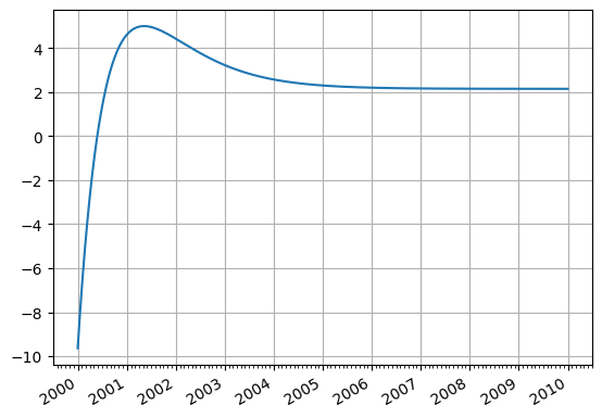
ns_curve = NelsonSiegelCurve(dt(2000, 1, 1), dt(2010, 1, 1), 0.03, -0.01, 0.01, 0.75)
solver = Solver(
    curves=[ns_curve],
    instruments=[
        IRS(dt(2000, 1, 1), "2y", "A", curves=ns_curve),
        IRS(dt(2000, 1, 1), "4y", "A", curves=ns_curve),
        IRS(dt(2000, 1, 1), "7y", "A", curves=ns_curve),
    ],
    s=[2.45, 2.90, 2.66],
    id="NS",
    instrument_labels=["2y", "4y", "7y"],
)

SUCCESS: `func_tol` reached after 8 iterations (levenberg_marquardt), `f_val`: 6.779292534286855e-13, `time`: 0.0312s

[9]:

ns_curve.plot("1b")

[9]:

(<Figure size 640x480 with 1 Axes>,
 <Axes: >,
 [<matplotlib.lines.Line2D at 0x1108d3750>])

Risk#

Since the Solver has been invoked all typically delta and gamma methods can now also be used against this curve risk model

[10]:

portfolio = IRS(dt(2003, 7, 1), "4y", "A", notional=50e6, fixed_rate=4.5, curves=ns_curve)
portfolio.delta(solver=solver)

[10]:

		local_ccy	usd
		display_ccy	usd
type	solver	label
instruments	NS	2y	-778.194724
		4y	-22432.219524
		7y	42449.616358

[11]:

portfolio.gamma(solver=solver)

[11]:

				type	instruments
				solver	NS
				label	2y	4y	7y
local_ccy	display_ccy	type	solver	label
usd	usd	instruments	NS	2y	1.183954	1.245186	-2.070988
				4y	1.245186	6.580990	-5.017871
				7y	-2.070988	-5.017871	-17.838847

[ ]:

Building Custom Curves (Nelson-Siegel)#

Nelson-Siegel Parametrization#

_BaseCurve ABCs#

The __getitem__ method#

Mutatbility and the Solver#

Risk#

This Page

The `getitem` method#

Mutatbility and the `Solver`#