
Multicurve Framework Construction#
The Solver is a generalised multi-variable solver targeting the
least squares problem. This means you can generally solve as many Curves/Surfaces as
necessary, with as many calibration Instruments as desired, with the following constraint:
Solving more variables, via more Instruments, simultaneously, is a harder problem and
costs performance.
Multi-curve frameworks are common in markets that either have multiple currencies, or multiple indexes. Examples are the EUR IR market which trades ESTR and Euribor (of various tenors), NOK, SEK, NZD and AUD, which also trade combinations of RFR indexes and tenor (IBOR-style) indexes.
This cookbook page will focus on NOK. Why? Because that market contains features which are useful to discuss and highlight in this article.
Warning
The Instruments configured in this article do not precisely match the NOK market, e.g. 3s6s basis is not a single currency basis swap (SBS) but is, in fact, a Spread of two IRSs. Configuring all of this correctly adds unnecessary coding verbosity to a tutorial page.
This cookbook page will not focus on: adding turns, or using different interpolation forms because these are covered in other cookbook articles.
There are currently two presented solutions in this article (although other solutions exist):
Adding all the instruments, all the curves and all market together into a single Solver and letting the optimisation algorithm run.
Identifying independence of curves, restructuring the instruments and using multiple, sequential solvers to improve performance.
Tradable instruments and data#
In NOK the common tradable instruments, and some of their features, are:
At the longer end (>3Y) IRSs indexed versus 6M-IBOR (NIBOR).
At the short end (<3Y) IRSs and FRAs indexed versus 3M-IBOR (NIBOR).
All products discounted with an RFR (NOWA) curve which has a relatively illiquid market although some ultra short prices are available, and other prices are modelled.
3s6s basis market trades across the curve.
3sRfr basis market trades across the curve.
We collect the following pricing data on 14th January 2025:
In [1]: data = DataFrame({
   ...:   "effective": [dt(2025, 1, 16), get_imm(code="h25"),  get_imm(code="m25"),  get_imm(code="u25"),  get_imm(code="z25"),
   ...:                 get_imm(code="h26"),  get_imm(code="m26"),  get_imm(code="u26"),  get_imm(code="z26"),
   ...:                 get_imm(code="h27"),  get_imm(code="m27"),  get_imm(code="u27"),  get_imm(code="z27")] + [dt(2025, 1, 16)] * 12,
   ...:   "termination": [None] + ["3m"] * 12 + ["4y", "5y", "6y", "7y", "8y", "9y", "10y", "12y", "15y", "20y", "25y", "30y"],
   ...:   "RFR": [4.50] + [None] * 24,
   ...:   "3m": [4.62, 4.45, 4.30, 4.19, 4.13, 4.07, 4.02, 3.98, 3.97, 3.91, 3.88, 3.855, 3.855, None, None, None, None, None, None, None, None, None, None, None, None],
   ...:   "6m": [4.62, None, None, None, None, None, None, None, None, None, None, None, None, 4.27, 4.23, 4.20, 4.19, 4.18, 4.17, 4.17, 4.14, 4.07, 3.94, 3.80, 3.66],
   ...:   "3s6s Basis": [None, 10.4, 10.4, 10.4, 10.4, 10.4, 10.4, 10.5, 10.5, 10.6, 10.6, 10.5, 10.5, 11.0, 10.9, 11.0, 11.2, 11.6, 12.1, 12.5, 13.8, 15, 16.3, 17.3, 17.8],
   ...:   "3sRfr Basis": [None] + [15.5] * 24,
   ...: })
   ...:

In [2]: data
Out[2]:
    effective termination  RFR   3m   6m  3s6s Basis  3sRfr Basis
0  2025-01-16        None 4.50 4.62 4.62         NaN          NaN
1  2025-03-19          3m  NaN 4.45  NaN       10.40        15.50
2  2025-06-18          3m  NaN 4.30  NaN       10.40        15.50
3  2025-09-17          3m  NaN 4.19  NaN       10.40        15.50
4  2025-12-17          3m  NaN 4.13  NaN       10.40        15.50
5  2026-03-18          3m  NaN 4.07  NaN       10.40        15.50
6  2026-06-17          3m  NaN 4.02  NaN       10.40        15.50
7  2026-09-16          3m  NaN 3.98  NaN       10.50        15.50
8  2026-12-16          3m  NaN 3.97  NaN       10.50        15.50
9  2027-03-17          3m  NaN 3.91  NaN       10.60        15.50
10 2027-06-16          3m  NaN 3.88  NaN       10.60        15.50
11 2027-09-15          3m  NaN 3.85  NaN       10.50        15.50
12 2027-12-15          3m  NaN 3.85  NaN       10.50        15.50
13 2025-01-16          4y  NaN  NaN 4.27       11.00        15.50
14 2025-01-16          5y  NaN  NaN 4.23       10.90        15.50
15 2025-01-16          6y  NaN  NaN 4.20       11.00        15.50
16 2025-01-16          7y  NaN  NaN 4.19       11.20        15.50
17 2025-01-16          8y  NaN  NaN 4.18       11.60        15.50
18 2025-01-16          9y  NaN  NaN 4.17       12.10        15.50
19 2025-01-16         10y  NaN  NaN 4.17       12.50        15.50
20 2025-01-16         12y  NaN  NaN 4.14       13.80        15.50
21 2025-01-16         15y  NaN  NaN 4.07       15.00        15.50
22 2025-01-16         20y  NaN  NaN 3.94       16.30        15.50
23 2025-01-16         25y  NaN  NaN 3.80       17.30        15.50
24 2025-01-16         30y  NaN  NaN 3.66       17.80        15.50
Single global solver#
The first thing that is possible is to structure and configure all of these instruments and data and insert them into a single global solver. There are 75 prices here; 25 for each curve. First we will construct the curves with node dates in fully consistent and recognisable positions, defined by the maturity dates of the general instruments.
In [3]: termination_dates = [add_tenor(row.effective, row.termination, "MF", "osl") for row in data.iloc[1:].itertuples()]

In [4]: data["termination_dates"] = [None] + termination_dates

# BUILD the Curves
In [5]: nowa = Curve(nodes={dt(2025, 1, 14): 1.0, dt(2025, 3, 19): 1.0, **{d: 1.0 for d in data.loc[1:, "termination_dates"]}}, convention="act365f", id="nowa", calendar="osl")

In [6]: nibor3 = Curve(nodes={dt(2025, 1, 14): 1.0, dt(2025, 3, 19): 1.0, **{d: 1.0 for d in data.loc[1:, "termination_dates"]}}, convention="act360", id="nibor3", calendar="osl")

In [7]: nibor6 = Curve(nodes={dt(2025, 1, 14): 1.0, dt(2025, 3, 19): 1.0, **{d: 1.0 for d in data.loc[1:, "termination_dates"]}}, convention="act360", id="nibor6", calendar="osl")
Deposit instruments#
Let’s build the deposit instruments:
# Instruments
In [8]: rfr_depo = [IRS(dt(2025, 1, 14), "1b", spec="nok_irs", curves="nowa")]

In [9]: ib3_depo = [IRS(dt(2025, 1, 16), "3m", spec="nok_irs3", curves=["nibor3", "nowa"])]

In [10]: ib6_depo = [IRS(dt(2025, 1, 16), "6m", spec="nok_irs6", curves=["nibor6", "nowa"])]

# Prices
In [11]: rfr_depo_s = [data.loc[0, "RFR"]]

In [12]: ib3_depo_s = [data.loc[0, "3m"]]

In [13]: ib6_depo_s = [data.loc[0, "6m"]]

# Labels
In [14]: rfr_depo_lbl = ["rfr_depo"]

In [15]: ib3_depo_lbl = ["3m_depo"]

In [16]: ib6_depo_lbl = ["6m_depo"]
Outright instruments#
Next we will build the 3m FRAs and the 6m swaps:
# Instruments
In [17]: ib3_fra = [FRA(row.effective, row.termination, spec="nok_fra3", curves=["nibor3", "nowa"]) for row in data.iloc[1:13].itertuples()]

In [18]: ib6_irs = [IRS(row.effective, row.termination, spec="nok_irs6", curves=["nibor6", "nowa"]) for row in data.iloc[13:].itertuples()]

# Prices
In [19]: ib3_fra_s = [_ for _  in data.loc[1:12, "3m"]]

In [20]: ib6_irs_s = [_ for _ in data.loc[13:, "6m"]]

# Labels
In [21]: ib3_fra_lbl = [f"fra_{i}" for i in range(1, 13)]

In [22]: ib6_irs_lbl = [f"irs_{i}" for i in range(1, 13)]
Basis instruments#
Now we add the 3s6s basis instruments as single currency basis swaps:
In [23]: sbs_irs = [SBS(row.effective, row.termination, spec="nok_sbs36", curves=["nibor3", "nowa", "nibor6", "nowa"]) for row in data.iloc[1:].itertuples()]

In [24]: sbs_irs_s = [_ for _ in data.loc[1:, "3s6s Basis"]]

In [25]: sbs_irs_lbl =  [f"sbs_{i}" for i in range(1, 25)]
And finally we add the 3sRfr basis instruments. There is not a default specification configured for this so we define our own.
In [26]: args = {
   ....:   'frequency': 'q',
   ....:   'stub': 'shortfront',
   ....:   'eom': False,
   ....:   'modifier': 'mf',
   ....:   'calendar': 'osl',
   ....:   'payment_lag': 0,
   ....:   'currency': 'nok',
   ....:   'convention': 'act360',
   ....:   'leg2_frequency': 'q',
   ....:   'leg2_convention': "act365f",
   ....:   'spread_compound_method': 'none_simple',
   ....:   'fixing_method': "ibor(2)",
   ....:   'leg2_spread_compound_method': 'none_simple',
   ....:   'leg2_fixing_method': 'rfr_payment_delay',
   ....:   'curves': ["nibor3", "nowa", "nowa", "nowa"],
   ....: }
   ....:

In [27]: sbs_rfr = [SBS(row.effective, row.termination, **args) for row in data.iloc[1:].itertuples()]

In [28]: sbs_rfr_s = [_ for _ in data.loc[1:, "3sRfr Basis"] * -1.0]

In [29]: sbs_rfr_lbl =  [f"sbs_rfr_{i}" for i in range(1, 25)]
Configuring the Solver#
We add all of the constructions into the Solver, and depending on the processor speed of the machine this might solve in 1-2 seconds.
In [30]: solver = Solver(
....: curves=[nibor3, nibor6, nowa],
....: instruments=rfr_depo + ib3_depo + ib6_depo + ib3_fra + ib6_irs + sbs_irs + sbs_rfr,
....: s = rfr_depo_s + ib3_depo_s + ib6_depo_s + ib3_fra_s + ib6_irs_s + sbs_irs_s + sbs_rfr_s,
....: instrument_labels = rfr_depo_lbl + ib3_depo_lbl + ib6_depo_lbl + ib3_fra_lbl + ib6_irs_lbl + sbs_irs_lbl + sbs_rfr_lbl,
....: )
....:
SUCCESS: `func_tol` reached after 7 iterations (levenberg_marquardt), `f_val`: 1.68013289759468e-12, `time`: 0.7399s
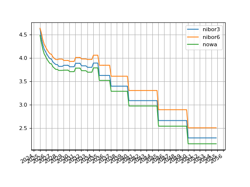
In [31]: nibor3.plot("3m", comparators=[nibor6, nowa], labels=["nibor3", "nibor6", "nowa"])
Out[31]:
(<Figure size 640x480 with 1 Axes>,
<Axes: >,
[<matplotlib.lines.Line2D at 0x14e487380>,
<matplotlib.lines.Line2D at 0x14e487230>,
<matplotlib.lines.Line2D at 0x14e4870e0>])
(Source code, png, hires.png, pdf)

Plotted 3m rates of each curve, NOWA, 3m-NIBOR and 6m-NIBOR.#
Independence and using multiple solvers#
Lets just reset the Curves for this next section.
In [32]: nowa = Curve(nodes={dt(2025, 1, 14): 1.0, dt(2025, 3, 19): 1.0, **{d: 1.0 for d in data.loc[1:, "termination_dates"]}}, convention="act365f", id="nowa", calendar="osl")

In [33]: nibor3 = Curve(nodes={dt(2025, 1, 14): 1.0, dt(2025, 3, 19): 1.0, **{d: 1.0 for d in data.loc[1:, "termination_dates"]}}, convention="act360", id="nibor3", calendar="osl")

In [34]: nibor6 = Curve(nodes={dt(2025, 1, 14): 1.0, dt(2025, 3, 19): 1.0, **{d: 1.0 for d in data.loc[1:, "termination_dates"]}}, convention="act360", id="nibor6", calendar="osl")
The “nowa” Curve is a primary curve in this scenario. Sometimes it is possible to refactor the market data quotes to obtain prices in Instruments impacting only one curve. This example does this in a slightly cavalier manner. In practice more care must be taken in the Instruments definitions to ensure the prices are exactly what is expected.
Here we will first solve the “nowa” Curve by extending the data table (in a simplistic manner), by subtracting the basis quotes from the outright quotes to obtain pure RFR rates. We will also do this to obtain 3m rates from 6m rates and vice-versa.
In [35]: data.loc[1:12, "RFR"] = data.loc[1:12, "3m"] - data.loc[1:12, "3sRfr Basis"] / 100.0

In [36]: data.loc[13:, "RFR"] = data.loc[13:, "6m"] - data.loc[13:, "3s6s Basis"] / 100.0 - data.loc[13:, "3sRfr Basis"] / 100.0

In [37]: data.loc[13:, "3m"] = data.loc[13:, "6m"] - data.loc[13:, "3s6s Basis"] / 100.0

In [38]: data.loc[1:12, "6m"] = data.loc[1:12, "3m"] + data.loc[1:12, "3s6s Basis"] / 100.0

In [39]: data
Out[39]:
    effective termination  RFR   3m   6m  3s6s Basis  3sRfr Basis termination_dates
0  2025-01-16        None 4.50 4.62 4.62         NaN          NaN               NaT
1  2025-03-19          3m 4.29 4.45 4.55       10.40        15.50        2025-06-19
2  2025-06-18          3m 4.14 4.30 4.40       10.40        15.50        2025-09-18
3  2025-09-17          3m 4.04 4.19 4.29       10.40        15.50        2025-12-17
4  2025-12-17          3m 3.98 4.13 4.23       10.40        15.50        2026-03-17
5  2026-03-18          3m 3.92 4.07 4.17       10.40        15.50        2026-06-18
6  2026-06-17          3m 3.86 4.02 4.12       10.40        15.50        2026-09-17
7  2026-09-16          3m 3.83 3.98 4.08       10.50        15.50        2026-12-16
8  2026-12-16          3m 3.82 3.97 4.08       10.50        15.50        2027-03-16
9  2027-03-17          3m 3.76 3.91 4.02       10.60        15.50        2027-06-17
10 2027-06-16          3m 3.73 3.88 3.99       10.60        15.50        2027-09-16
11 2027-09-15          3m 3.70 3.85 3.96       10.50        15.50        2027-12-15
12 2027-12-15          3m 3.70 3.85 3.96       10.50        15.50        2028-03-15
13 2025-01-16          4y 4.00 4.16 4.27       11.00        15.50        2029-01-16
14 2025-01-16          5y 3.97 4.12 4.23       10.90        15.50        2030-01-16
15 2025-01-16          6y 3.94 4.09 4.20       11.00        15.50        2031-01-16
16 2025-01-16          7y 3.92 4.08 4.19       11.20        15.50        2032-01-16
17 2025-01-16          8y 3.91 4.06 4.18       11.60        15.50        2033-01-17
18 2025-01-16          9y 3.89 4.05 4.17       12.10        15.50        2034-01-16
19 2025-01-16         10y 3.89 4.04 4.17       12.50        15.50        2035-01-16
20 2025-01-16         12y 3.85 4.00 4.14       13.80        15.50        2037-01-16
21 2025-01-16         15y 3.77 3.92 4.07       15.00        15.50        2040-01-16
22 2025-01-16         20y 3.62 3.78 3.94       16.30        15.50        2045-01-16
23 2025-01-16         25y 3.47 3.63 3.80       17.30        15.50        2050-01-17
24 2025-01-16         30y 3.33 3.48 3.66       17.80        15.50        2055-01-18
Preliminary Solver#
Then we can create a Solver which solves the NOWA curve directly:
In [40]: solver1 = Solver(
   ....:   curves=[nowa],
   ....:   instruments=rfr_depo + [IRS(row.effective, row.termination, spec="nok_irs", curves="nowa") for row in data.iloc[1:].itertuples()],
   ....:   s = rfr_depo_s + [row.RFR for row in data.iloc[1:].itertuples()],
   ....: )
   ....:
SUCCESS: `func_tol` reached after 7 iterations (levenberg_marquardt), `f_val`: 1.1515659305059484e-16, `time`: 0.0507s
Additional Solvers in dependency chain#
This Curve is now available to use to price the remaining Curves.
We will do the same trick for the rates on the 3M curve.
Notice that we use the pre_solvers input to pass the already solved Curve into the system.
In [41]: solver2 = Solver(
   ....:   pre_solvers=[solver1],
   ....:   curves=[nibor3],
   ....:   instruments=ib3_depo + ib3_fra + [IRS(row.effective, row.termination, spec="nok_irs3", curves=["nibor3", "nowa"]) for row in data.iloc[13:].itertuples()],
   ....:   s = ib3_depo_s + ib3_fra_s + [row._4 for row in data.iloc[13:].itertuples()],
   ....: )
   ....:
SUCCESS: `func_tol` reached after 7 iterations (levenberg_marquardt), `f_val`: 6.682431122442255e-17, `time`: 0.1952s
And finally we repeat this for the 6M Nibor curve. Notice that the total time to solve is about 50% of the time taken by the single solver system.
In [42]: solver3 = Solver(
   ....:   pre_solvers=[solver2],
   ....:   curves=[nibor6],
   ....:   instruments=ib6_depo + [IRS(row.effective, row.termination, spec="nok_irs6", curves=["nibor6", "nowa"]) for row in data.iloc[1:13].itertuples()] + ib6_irs,
   ....:   s = ib6_depo_s + [row._5 for row in data.iloc[1:13].itertuples()] + ib6_irs_s,
   ....: )
   ....:
SUCCESS: `func_tol` reached after 7 iterations (levenberg_marquardt), `f_val`: 6.57458899093436e-17, `time`: 0.1126s
We can plot the curves.
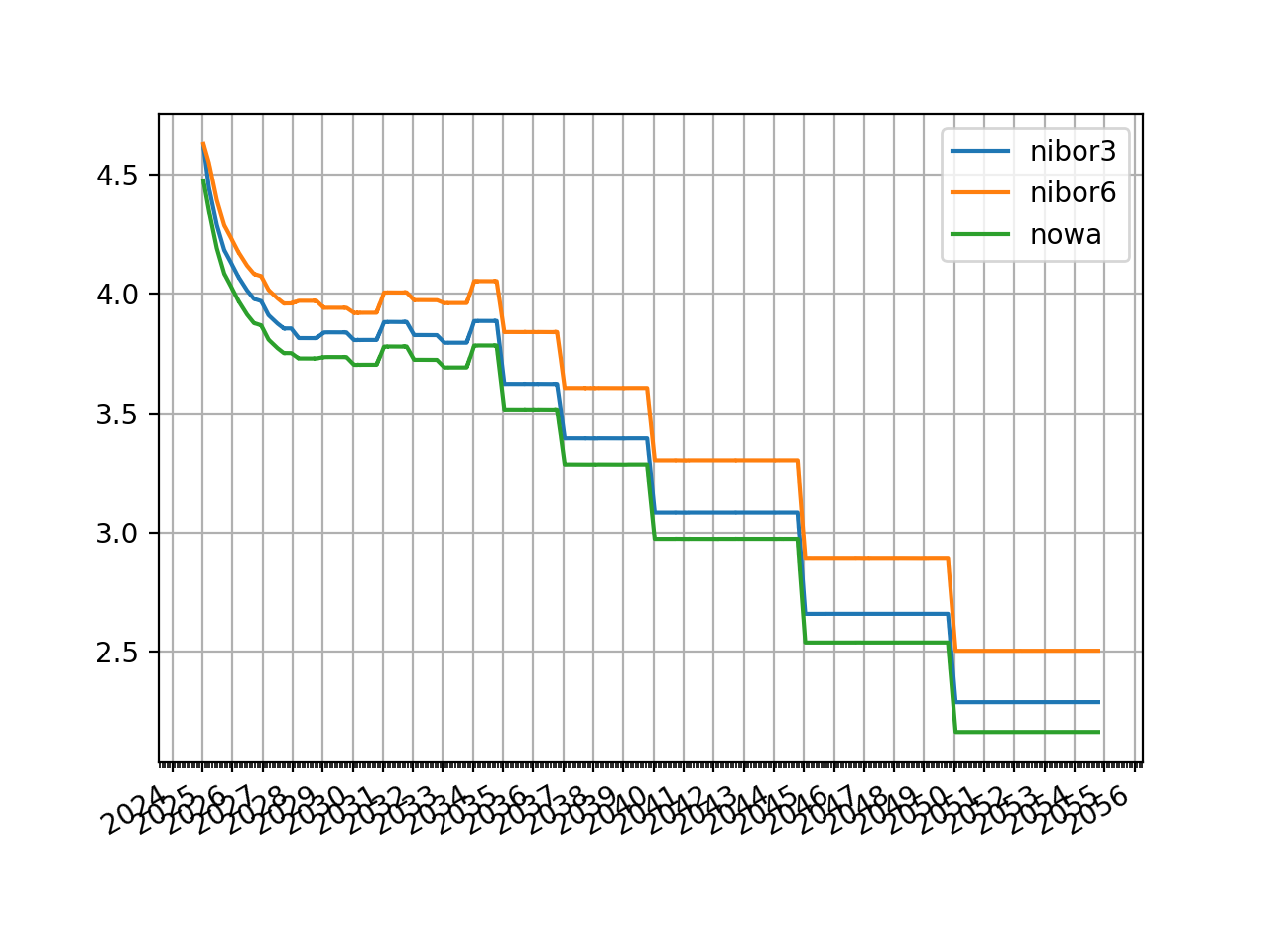
In [43]: nibor3.plot("3m", comparators=[nibor6, nowa], labels=["nibor3", "nibor6", "nowa"])
Out[43]:
(<Figure size 640x480 with 1 Axes>,
 <Axes: >,
 [<matplotlib.lines.Line2D at 0x13bc6a120>,
  <matplotlib.lines.Line2D at 0x13bc6a270>,
  <matplotlib.lines.Line2D at 0x13bc6a3c0>])
(Source code, png, hires.png, pdf)

Plotted 3m rates of each curve, NOWA, 3m-NIBOR and 6m-NIBOR.#
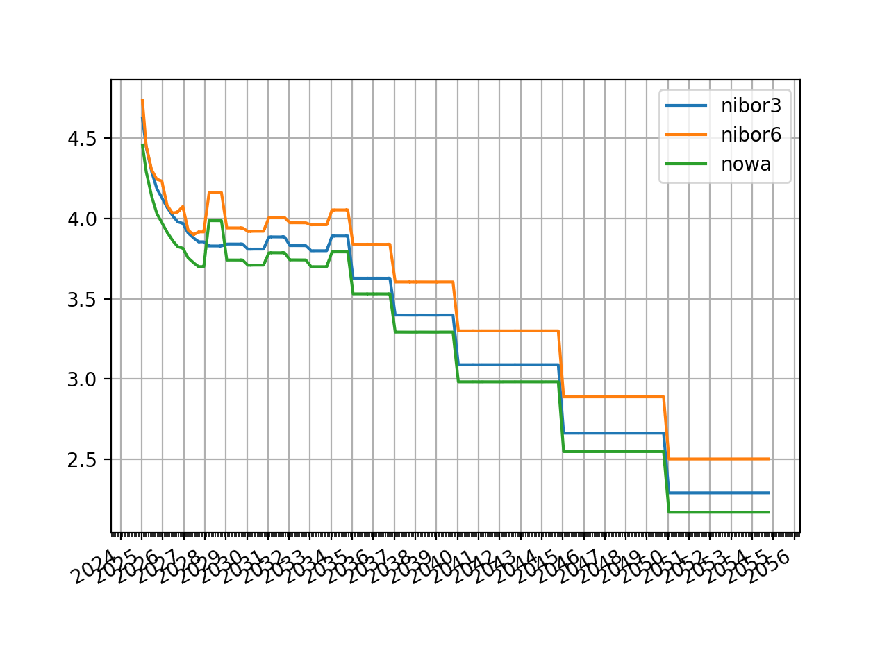
The curves look different, and erroneous. This is not because of the method used: i.e. the alternative framework and independent solvers. It is because the operation of adding the basis to imply rates of alternative Instruments is not exact, in this case, and was too simplistic. A 3s6s SBS rate of 3m-NIBOR + 10bps does not equate to subtracting 10bps from the fixed rate of a 6m IRS to yield a 3m IRS fixed rate, because the frequencies (“A”, “S” and “Q”) do not align and the conventions (“30e360” and “Act360”) do not align either. This is also a problem for the RFR basis which has a convention of “Act365F” whilst the IBOR type is “Act360”. This approximation has created kinks about the part of the curve where real prices cross-over to approximated ones.