
FX Vol Smiles & Surfaces#
The rateslib.fx_volatility module includes classes for Smiles and Surfaces
which can be used to price FX Options and FX Option Strategies.
Create an FX Volatility Smile at a given expiry indexed by delta percent. |
|
|
Create an FX Volatility Smile at a given expiry indexed by strike using SABR parameters. |
Create an FX Volatility Surface parametrised by cross-sectional Smiles at different expiries. |
|
|
Create an FX Volatility Surface parametrised by cross-sectional Smiles at different expiries. |
Introduction and FX Volatility Smiles#
Ratelib offers two different Smile models for pricing FX volatility at a given expiry. An
FXDeltaVolSmile and an
FXSabrSmile.
The FXDeltaVolSmile is parametrised by a series of
(delta-index, vol) node points interpolated by a natural cubic spline. This interpolation is
automatically constructed with knot sequences that adjust to the number of given nodes:
Providing only one node, e.g. (0.5, 11.0), will create a constant volatility level, here at 11%.
Providing two nodes, e.g. (0.25, 8.0), (0.75, 10.0) will create a straight line gradient across the whole delta axis, here rising by 1% volatility every 0.25 in delta-index.
Providing more nodes (appropriately calibrated) will create a traditional smile shape with the mentioned interpolation structure.
An FXDeltaVolSmile must also be initialised with a delta_type to define how it references
delta on its index. It can still be used to price Instruments even
if their delta types are different. That is, an FXDeltaVolSmile defined by “forward” delta
types can still price FXOptions defined with “spot” delta types or premium adjusted
delta types due to appropriate mathematical conversions.
An FXSabrSmile is a Smile parametrised by the
conventional \(\alpha, \beta, \rho, \nu\) variables of the SABR model. The parameter
\(\beta\) is considered a hyper-parameter and will not be varied by a
Solver but \(\alpha, \rho, \nu\) will be varied.
Both Smiles must also be initialised with:
An
eval_datewhich serves the same purpose as the initial node point on a Curve, and indicates ‘today’ or ‘horizon’.An
expiry, for which options priced with this Smile must have an equivalent expiry or errors will be raised.
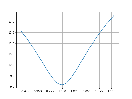
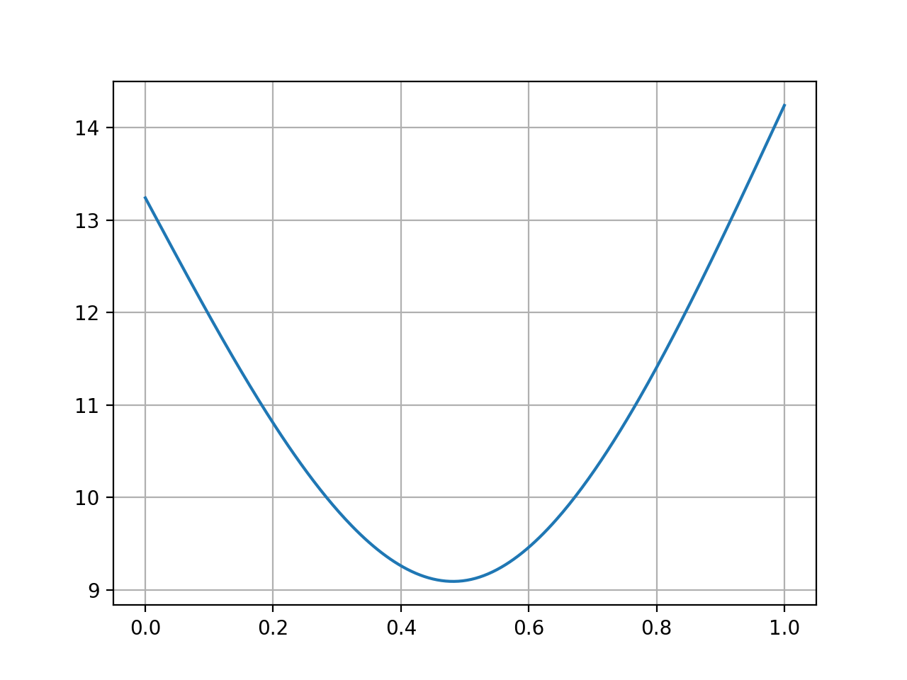
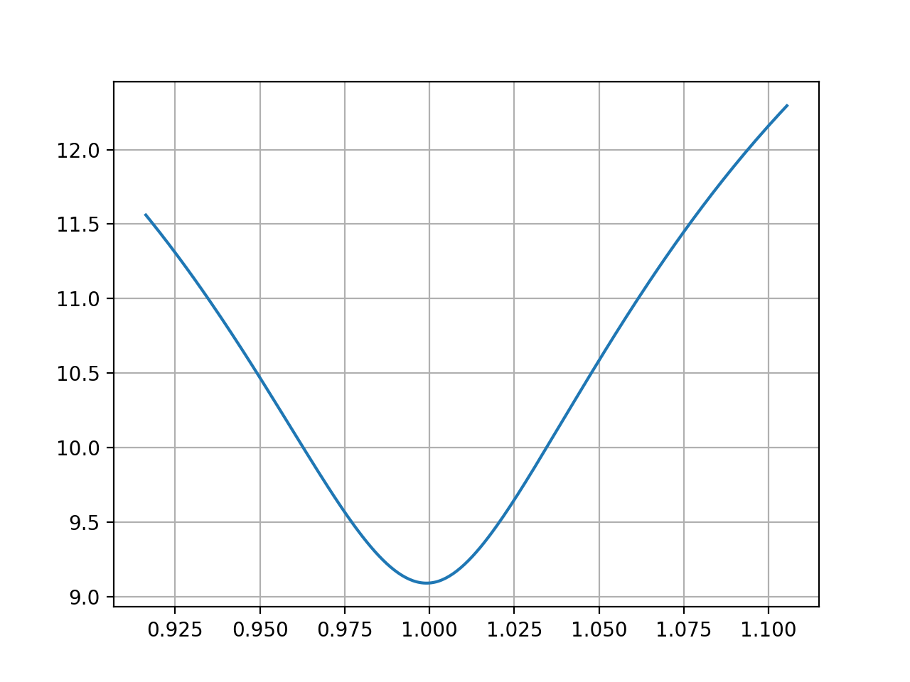
An example of an FXDeltaVolSmile is shown below.
In [1]: smile = FXDeltaVolSmile(
   ...:     eval_date=dt(2000, 1, 1),
   ...:     expiry=dt(2000, 7, 1),
   ...:     nodes={
   ...:         0.25: 10.3,
   ...:         0.5: 9.1,
   ...:         0.75: 10.8
   ...:     },
   ...:     delta_type="forward"
   ...: )
   ...:

#  -->  smile.plot()
#  -->  smile.plot(x_axis="moneyness")

Constructing a Smile#
It is expected that Smiles will typically be calibrated to market prices, similar to interest rate curves.
The following data describes Instruments to calibrate the EURUSD FX volatility surface on 7th May 2024. We will take a cross-section of this data, at the 3-week expiry (28th May 2024), and create both an FXDeltaVolSmile and FXSabrSmile.
FX Options are multi-currency derivative Instruments and require an FXForwards
framework for pricing. We will do this first using other prevailing market data,
i.e. local currency interest rates at 3.90% and 5.32%, and an FX Swap rate at 8.85 points.
# Define the interest rate curves for EUR, USD and X-Ccy basis
In [2]: usdusd = Curve({dt(2024, 5, 7): 1.0, dt(2024, 5, 30): 1.0}, calendar="nyc", id="usdusd")

In [3]: eureur = Curve({dt(2024, 5, 7): 1.0, dt(2024, 5, 30): 1.0}, calendar="tgt", id="eureur")

In [4]: eurusd = Curve({dt(2024, 5, 7): 1.0, dt(2024, 5, 30): 1.0}, id="eurusd")

# Create an FX Forward market with spot FX rate data
In [5]: fxf = FXForwards(
   ...:     fx_rates=FXRates({"eurusd": 1.0760}, settlement=dt(2024, 5, 9)),
   ...:     fx_curves={"eureur": eureur, "usdusd": usdusd, "eurusd": eurusd},
   ...: )
   ...:

In [6]: pre_solver = Solver(
   ...:     curves=[eureur, eurusd, usdusd],
   ...:     instruments=[
   ...:         IRS(dt(2024, 5, 9), "3W", spec="eur_irs", curves="eureur"),
   ...:         IRS(dt(2024, 5, 9), "3W", spec="usd_irs", curves="usdusd"),
   ...:         FXSwap(dt(2024, 5, 9), "3W", pair="eurusd", curves=["eurusd", "usdusd"]),
   ...:     ],
   ...:     s=[3.90, 5.32, 8.85],
   ...:     fx=fxf,
   ...:     id="rates_sv",
   ...: )
   ...:
SUCCESS: `func_tol` reached after 2 iterations (levenberg_marquardt), `f_val`: 9.01049134669041e-13, `time`: 0.0012s
Since EURUSD Options are not premium adjusted and the premium currency is USD we will match
the FXDeltaVolSmile with this definition and set it to a delta_type of ‘spot’, matching
the market convention of these quoted instruments.
Since we have 5 calibrating instruments we can safely utilise 5 degrees of freedom.
In [7]: dv_smile = FXDeltaVolSmile(
   ...:     nodes={
   ...:         0.10: 10.0,
   ...:         0.25: 10.0,
   ...:         0.50: 10.0,
   ...:         0.75: 10.0,
   ...:         0.90: 10.0,
   ...:     },
   ...:     eval_date=dt(2024, 5, 7),
   ...:     expiry=dt(2024, 5, 28),
   ...:     delta_type="spot",
   ...:     id="eurusd_3w_smile"
   ...: )
   ...:

In [8]: sabr_smile = FXSabrSmile(
   ...:     nodes={
   ...:         "alpha": 0.10,  # default vol level set to 10%
   ...:         "beta": 1.0,  # model is fully lognormal
   ...:         "rho": 0.10,
   ...:         "nu": 1.0,  # initialised with curvature
   ...:     },
   ...:     eval_date=dt(2024, 5, 7),
   ...:     expiry=dt(2024, 5, 28),
   ...:     id="eurusd_3w_smile"
   ...: )
   ...:
The above FXDeltaVolSmile is initialised as a flat vol at 10%, whilst the FXSabrSmile is initialised with around 10% with some shallow curvature. In order to calibrate these, we need to create the pricing instruments, given in the market prices data table.
# Setup the Solver instrument calibration for FXOptions and vol Smiles
In [9]: option_args=dict(
   ...:     pair="eurusd", expiry=dt(2024, 5, 28), calendar="tgt|fed", delta_type="spot",
   ...:     curves=["eurusd", "usdusd"], vol="eurusd_3w_smile"
   ...: )
   ...:

In [10]: dv_solver = Solver(
   ....:     pre_solvers=[pre_solver],
   ....:     curves=[dv_smile],
   ....:     instruments=[
   ....:         FXStraddle(strike="atm_delta", **option_args),
   ....:         FXRiskReversal(strike=("-25d", "25d"), **option_args),
   ....:         FXRiskReversal(strike=("-10d", "10d"), **option_args),
   ....:         FXBrokerFly(strike=(("-25d", "25d"), "atm_delta"), **option_args),
   ....:         FXBrokerFly(strike=(("-10d", "10d"), "atm_delta"), **option_args),
   ....:     ],
   ....:     s=[5.493, -0.157, -0.289, 0.071, 0.238],
   ....:     fx=fxf,
   ....:     id="dv_solver",
   ....: )
   ....:
SUCCESS: `func_tol` reached after 11 iterations (levenberg_marquardt), `f_val`: 1.710466169564503e-16, `time`: 0.0321s
The FXSabrSmile can be similarly calibrated.
In [11]: sabr_solver = Solver(
....: pre_solvers=[pre_solver],
....: curves=[sabr_smile],
....: instruments=[
....: FXStraddle(strike="atm_delta", **option_args),
....: FXRiskReversal(strike=("-25d", "25d"), **option_args),
....: FXRiskReversal(strike=("-10d", "10d"), **option_args),
....: FXBrokerFly(strike=(("-25d", "25d"), "atm_delta"), **option_args),
....: FXBrokerFly(strike=(("-10d", "10d"), "atm_delta"), **option_args),
....: ],
....: s=[5.493, -0.157, -0.289, 0.071, 0.238],
....: fx=fxf,
....: id="sabr_solver",
....: )
....:
SUCCESS: `conv_tol` reached after 12 iterations (levenberg_marquardt), `f_val`: 8.325531146469465e-05, `time`: 0.0684s
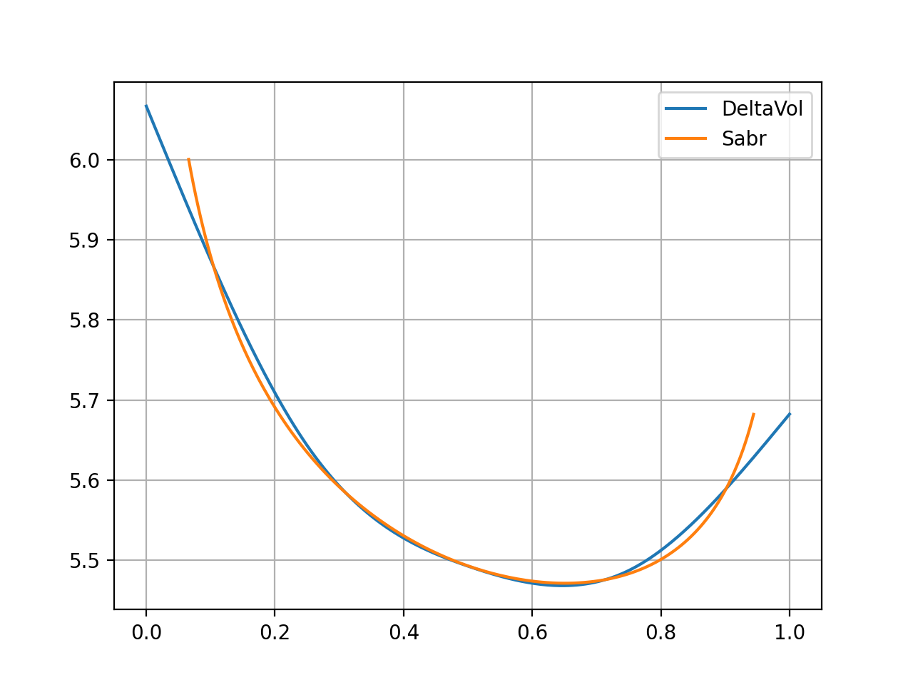
In [12]: dv_smile.plot(f=fxf.rate("eurusd", dt(2024, 5, 30)), x_axis="delta", labels=["DeltaVol", "Sabr"])
Out[12]:
(<Figure size 640x480 with 1 Axes>,
<Axes: >,
[<matplotlib.lines.Line2D at 0x13f796270>])
(Source code, png, hires.png, pdf)
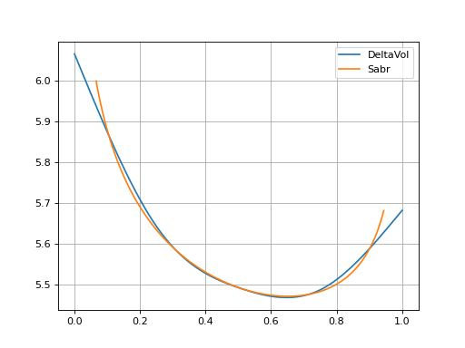
Rateslib Vol Smile: ‘delta index’#
FX Volatility Surfaces#
An FXDeltaVolSurface in rateslib is a collection of
multiple, cross-sectional FXDeltaVolSmile where:
each cross-sectional Smile will represent a DeltaVolSmile at that explicit expiry,
the delta type and the delta indexes on each cross-sectional Smile are the same,
each Smile has its own calibrated node values,
Smiles for expiries that do not pre-exist are generated with an interpolation scheme that uses linear total variance, which is equivalent to flat-forward volatility, measured relative to the delta indexes.
An FXSabrSurface is a collection of multiple,
cross-sectional FXSabrSmile where:
each cross-sectional Smile will represent a SabrSmile at that explicit expiry,
each cross-sectional Smile is defined by its own \(\alpha, \beta, \rho, \nu\) parameters,
Smiles for expiries that do not pre-exist are not generated. Volatility values for a given strike are interpolated with linear total variance between the volatility on neighboring Smiles for the same strike.
Further Information
Examples of the differences between each Surface type, temporal interpolation and using volatility weights and calibrating an entire EURUSD surface to all given market data is included in three separate notebooks available in the Cookbook.
Comparing Surface Interpolation for FX Options.
FX Volatility Surface Temporal Interpolation.
A EURUSD market for IRS, cross-currency and FX volatility.