
Replicating a Pfizer Default Curve & CDS#
The raw data necessary to build the curves and replicate the pricing of Pfizer CDS is added to Python.
In [1]: irs_tenor = ["1m", "2m", "3m", "6m", "12m", "2y", "3y", "4y", "5y", "6y", "7y", "8y", "9y", "10y", "12y"]

In [2]: irs_rates = [4.8457, 4.7002, 4.5924, 4.3019, 3.8992, 3.5032, 3.3763, 3.3295, 3.3165, 3.3195, 3.3305, 3.3450, 3.3635, 3.3830, 3.4245]

In [3]: cds_tenor = ["6m", "12m", "2y", "3y", "4y", "5y", "7y", "10y"]

In [4]: cds_rates = [0.11011, 0.14189, 0.20750, 0.26859, 0.32862, 0.37861, 0.51068, 0.66891]
Since the SOFR curve is a rates component, independent from the Pfizer credit component, we will build that, separately, first. This is no different to any of the other tutorials or examples constructing a basic SOFR curve - it places node dates at the maturity of each IRS and solves the curve with exact precision.
In [5]: today = dt(2024, 10, 4)  # Friday 4th October 2024

In [6]: spot = dt(2024, 10, 8)  # Tuesday 8th October 2024

In [7]: disc_curve = Curve(
   ...:     nodes={
   ...:         today: 1.0,
   ...:         **{add_tenor(spot, _, "mf", "nyc"): 1.0 for _ in irs_tenor}
   ...:     },
   ...:     calendar="nyc",
   ...:     convention="act360",
   ...:     interpolation="log_linear",
   ...:     id="sofr"
   ...: )
   ...:

In [8]: us_rates_sv = Solver(
   ...:     curves=[disc_curve],
   ...:     instruments=[
   ...:         IRS(spot, _, spec="usd_irs", curves="sofr") for _ in irs_tenor
   ...:     ],
   ...:     s=irs_rates,
   ...:     instrument_labels=irs_tenor,
   ...:     id="us_rates"
   ...: )
   ...:
SUCCESS: `func_tol` reached after 6 iterations (levenberg_marquardt), `f_val`: 2.5124140142870088e-15, `time`: 0.1071s
This framework for:
firstly, structuring a Curve with chosen hyper-parameters such as nodes, interpolation, etc.,
secondly, calibrating that Curve with a chosen set of market Instruments,
should now be familiar. Here we will create a hazard Curve for Pfizer using node dates at constant tenor points (notice these are not the maturity of the so called credit-imm dates - but they could be if you wanted) and then calibrate the curve with proper CDS market instruments and prices.
In [9]: cds_eff = dt(2024, 9, 20)

In [10]: cds_mats = [add_tenor(dt(2024, 12, 20), _, "mf", "all") for _ in cds_tenor]

In [11]: hazard_curve = Curve(
   ....:     nodes={
   ....:         today: 1.0,
   ....:         **{add_tenor(spot, _, "mf", "nyc"): 1.0 for _ in cds_tenor}
   ....:     },
   ....:     calendar="all",
   ....:     convention="act365f",
   ....:     interpolation="log_linear",
   ....:     id="pfizer"
   ....: )
   ....:

In [12]: pfizer_sv = Solver(
   ....:     curves=[hazard_curve],
   ....:     pre_solvers=[us_rates_sv],
   ....:     instruments=[
   ....:         CDS(cds_eff, _, spec="us_ig_cds", curves=["pfizer", "sofr"]) for _ in cds_mats
   ....:     ],
   ....:     s=cds_rates,
   ....:     instrument_labels=cds_tenor,
   ....:     id="pfizer_cds"
   ....: )
   ....:
SUCCESS: `func_tol` reached after 6 iterations (levenberg_marquardt), `f_val`: 6.2704010989490665e-12, `time`: 0.1681s
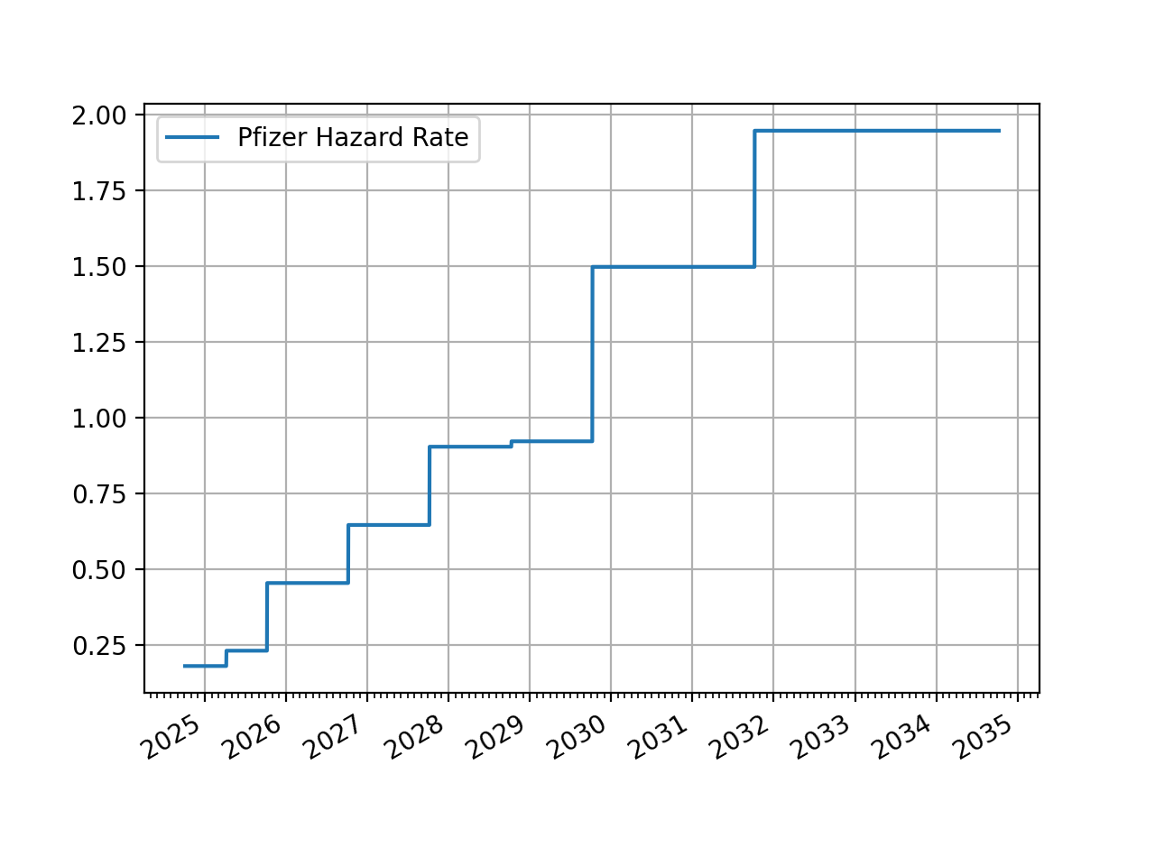
Lets look at the structure of the hazard rates generated. To do this we plot the ‘1d’ overnight rates of the ‘pfizer’ hazard curve.
In [13]: hazard_curve.plot("1d")
Out[13]:
(<Figure size 640x480 with 1 Axes>,
 <Axes: >,
 [<matplotlib.lines.Line2D at 0x11c05a0d0>])
(Source code, png, hires.png, pdf)

By definition, the probabilities of survival are calculable directly from the hazard Curve.
In [14]: hazard_curve[dt(2025, 10, 4)]  # Probability Pfizer survives at least 1yr.
Out[14]: <Dual: 0.997942, (pfizer0, pfizer1, pfizer2, ...), [0.0, 0.0, 1.0, ...]>

In [15]: hazard_curve[dt(2029, 10, 4)]  # Probability Pfizer survives at least 5yr.
Out[15]: <Dual: 0.969182, (pfizer0, pfizer1, pfizer2, ...), [0.0, 0.0, 0.0, ...]>

In [16]: hazard_curve[dt(2034, 10, 4)]  # Probability Pfizer survives at least 10yr.
Out[16]: <Dual: 0.887254, (pfizer0, pfizer1, pfizer2, ...), [0.0, 0.0, 0.0, ...]>
Pricing and risk metrics are calculable within rateslib’s natural framework. Let’s build the traditional 5Y Pfizer CDS.
In [17]: cds = CDS(
   ....:     effective=dt(2024, 9, 20),
   ....:     termination=dt(2029, 12, 20),
   ....:     spec="us_ig_cds",
   ....:     curves=["pfizer", "sofr"],
   ....:     notional=10e6,
   ....: )
   ....:

In [18]: cds.rate(solver=pfizer_sv)  # this compares to BBG: "Trd Sprd (bp)"
Out[18]: <Dual: 0.378610, (sofr0, sofr1, sofr2, ...), [0.0, 0.0, -0.0, ...]>

In [19]: cds.npv(solver=pfizer_sv)  # this compares to BBG: "Cash Amount"
Out[19]: <Dual: -298463.114836, (pfizer0, pfizer1, pfizer2, ...), [5915513.8, -161421.6, -210720.6, ...]>

In [20]: cds.analytic_delta(hazard_curve, disc_curve)
Out[20]: <Dual: 4803.153679, (pfizer0, pfizer1, pfizer2, ...), [159.0, 488.6, 725.2, ...]>

In [21]: cds.accrued(dt(2024, 10, 7))  # this is 17 days of accrued
Out[21]: -4722.222222222222

In [22]: cds.delta(solver=pfizer_sv).groupby("solver").sum()  # this compares to: "Spread DV01" and "IR DV01"
Out[22]:
local_ccy       usd
display_ccy     usd
solver
pfizer_cds  4930.82
us_rates      76.82
Whe can also show the analytic risk if the recovery rate is increased by 1%. This is the PnL purely for this contract.
In [23]: cds.analytic_rec_risk(hazard_curve, disc_curve)
Out[23]: -3030.8708850230523
This does not compare with other systems Rec Risk (1%) of 78.75. To understand and return this value consider the follow up cookbook article what are exogenous variables?.