SmithWilsonCurve

class rateslib.curves.academic.SmithWilsonCurve(nodes, ufr, solve_alpha=False, id=NoInput.blank, *, convention=NoInput.blank, modifier=NoInput.blank, calendar=NoInput.blank, ad=0, index_base=NoInput.blank, index_lag=NoInput.blank, collateral=NoInput.blank, credit_discretization=NoInput.blank, credit_recovery_rate=NoInput.blank)

Bases: _WithMutability, _BaseCurve

A Smith-Wilson style Curve defined by discount factors.

The discount factors on this curve are defined by:

\[v(t) = e^{-wt} + \mathbf{W}[t, \mathbf{u}] \mathbf{\hat{b}}\]

where,

\[\begin{split}W(t, u) &= e^{-w(t+u)} \left ( \alpha \min(t, u) - e^{\alpha max(t, u)} sinh(\alpha min(t, u)) \right ) \\ w &= \ln ( 1 + UFR)\end{split}\]

and \(\alpha\) and \(UFR\) are parameters controlling convergence to some rate in the long term, and \(\mathbf{\hat{b}}\) are calibration parameters. All ‘time’ quantities are derived under an effective ‘Act/365.25’ day count convention.

Parameters:

• nodes (dict[datetime, float]) – The parameters of the Curve. The value associated with the initial node date is treated as \(\alpha\). All subsequent key-value pairs define the (Mx1) vectors \(\mathbf{u}\) and \(\mathbf{\hat{b}}\) respectively.

• ufr (float, required) – The rates that is denoted by the ‘ultimate forward rate’.

• solve_alpha (bool, optional (set as False)) – Define whether \(\alpha\) is to be treated as a parameter in the solver process simultaneously with \(\mathbf{\hat{b}}\).

• id (str, optional (set randomly)) – The unique identifier to distinguish between curves in a multicurve framework.

• convention (Convention, str, optional (set as Act365_25)) – The convention of the curve for determining rates. Please see dcf() for all available options.

• modifier (str, optional (set by ‘defaults’)) – The modification rule, in {“F”, “MF”, “P”, “MP”}, for determining rates when input as a tenor, e.g. “3M”.

• calendar (calendar, str, optional (set as ‘all’)) – The holiday calendar object to use. If str, looks up named calendar from static data. Used for determining rates.

• ad (int in {0, 1, 2}, optional) – Sets the automatic differentiation order. Defines whether to convert node values to float, Dual or Dual2. It is advised against using this setting directly. It is mainly used internally.

• index_base (float, optional) – The initial index value at the initial node date of the curve. Used for forecasting future index values.

• index_lag (int, optional (set by ‘defaults’)) – Number of months of by which the index lags the date. For example if the initial curve node date is 1st Sep 2021 based on the inflation index published 17th June 2023 then the lag is 3 months. Best practice is to use 0 months.

• collateral (str, optional (set as None)) – A currency identifier to denote the collateral currency against which the discount factors for this Curve are measured.

• credit_discretization (int, optional (set by ‘defaults’)) – A parameter for numerically solving the integral for credit protection legs and default events. Expressed in calendar days. Only used by Curves functioning as hazard Curves.

• credit_recovery_rate (Variable | float, optional (set by ‘defaults’)) – A parameter used in pricing credit protection legs and default events.

Notes

EIOPA’s Approach

The Smith-Wilson Curve as defined by EIOPA is a Curve designed with the following properties:

• A matrix-type formulation to solve calibration parameters using linear algebra.

• An ‘ultra-forward-rate (UFR)’ and convergence parameter \(\alpha\) to control the curve beyond points at which there might be priced market instruments.

The official version of the Smith-Wilson discount factor function is:

\[v(t) = e^{-wt} + \mathbf{W}[t, \mathbf{u}]\mathbf{C} \mathbf{b}\]

In this equation a set of N bonds (likely coupon bearing) are selected from the market and the vector \(\mathbf{u}\), of length M, contains ordered times to each cashflow of any bond. The (MxN) matrix \(\mathbf{C}_{i,j}\) structures individual cashflows attributable to each bond, j, at cashflow date, \(u_i\). And \(\mathbf{b}\), the calibration parameters, must have length N.

The Smith-Wilson concept is to use that same equation replacing, t, with each \(u_i\), and then multiplying each cashflow of any bond by those relevant discount factors to return the market price, \(\mathbf{p}\), i.e.

\[\mathbf{p} = \mathbf{C^T} v[\mathbf{u}] = \mathbf{C^T} e^{-w\mathbf{u}} + \mathbf{C^T W[u,u] C b}\]

After this is rearranged it yields,

\[\mathbf{b} = \left ( \mathbf{C^T W[u,u] C} \right )^{-1} ( \mathbf{p} - \mathbf{C^T} e^{-w \mathbf{u}} )\]

which is transformable into the equations recognisable in the EIOPA document using their same substitutions,

\[\begin{split}\mathbf{b} &= \left ( \mathbf{Q^T H[u,u] Q} \right )^{-1} ( \mathbf{p} - \mathbf{q} ) \\ \mathbf{d} &= e^{-w \mathbf{u}} \\ \mathbf{Q} &= \mathbf{d_\Delta C} \\ \mathbf{W[u,u]} &= \mathbf{d_\Delta H[u,u] d_\Delta} \\ \mathbf{q} &= \mathbf{C^T d} \\\end{split}\]

Rateslib’s Approach

Rateslib makes two key changes. Firstly it recognises that for an unchanged \(\mathbf{u}\) vector, i.e. the cashflow dates remain the same, and unchanged discount factors at those dates, i.e. unchanged \(v[\mathbf{u}]\) the system can be equivalently formulated in terms of zero coupon bonds, so that:

\[\underbrace{\mathbf{C b}}_{(M \times N) (N \times 1)} = \underbrace{\mathbf{I \hat{b}}}_{(M \times M) (M \times 1)}\]

Since the market prices of the bonds are known and the discount factors of these synthesised zero coupon bonds are not known apriori this transformation does not allow the linear algebraic solution (EIOPA’s approach) to remain viable. That leads to the second change.

Rateslib does not bootstrap or algebraically solve Curves. It uses a global solver. This is why the above change is permissible because even under the reformulation it will still converge on a solution for \(\mathbf{\hat{b}}\) which reprices the bonds.

Implication

The general rules for Curve solving remain applicable; if M > N then the system is underspecified and may result in spurious behavior. If M = N and maturities are all appropriately chosen the solution is exact and unique.

Because rateslib treats Curve parameterization and Instrument calibration as two separate processes there is increased flexibility in both aspects. The calibrating bonds do not necessarily have to match the nodes of the Smith-Wilson Curve. Under EIOPA’s approach this is obviously not possible because the framework of equations relies on setting up the appropriate cashflow matrix and array of cashflow dates.

Note

Rateslib will not determine the matrices \(\mathbf{W[u,u], H[u,u], Q, C}\) etc. becuase its methods does not require them

Examples

The standard EIOPA example happens to include a 20x20 cashflow matrix, each bond valued at par with increasing coupon rates, implying increasing YTM.

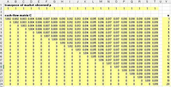
Because this is a square matrix and satisfies the criteria above the rateslib solution will match EIOPA’s.

In [1]: sw = SmithWilsonCurve(
   ...:     nodes={
   ...:         dt(2000, 1, 1): 0.12376,       #  <--  alpha value used in EIOPA file
   ...:         **{dt(2000+i, 1, 1): 0.1 for i in range(1, 21)}
   ...:     },
   ...:     solve_alpha=False,
   ...:     ufr= 4.2,
   ...:     id="academic_curve",
   ...: )
   ...: 

In [2]: coupons = [0.2, 0.225, 0.3, 0.425, 0.55, 0.7, 0.85, 1.0, 1.15, 1.275, 1.4, 1.475, 1.575, 1.65, 1.7, 1.75, 1.8, 1.825, 1.85, 1.875]

In [3]: bonds = [
   ...:     FixedRateBond(
   ...:         effective=dt(2000, 1, 1),
   ...:         termination=f"{i}Y",         #  <-  1Y to 20Y
   ...:         fixed_rate=coupons[i-1],     #  <-  Coupons as specified
   ...:         calendar="all",
   ...:         ex_div=1,
   ...:         convention="actacticma",
   ...:         frequency="A",
   ...:         curves="academic_curve",
   ...:         metric="dirty_price"
   ...:     )
   ...:     for i in range(1, 21)
   ...: ]
   ...: 

In [4]: prices = [100.0] * 20                #  <-  All bonds priced to par

In [5]: Solver(curves=[sw], instruments=bonds, s=prices)
SUCCESS: `func_tol` reached after 18 iterations (levenberg_marquardt), `f_val`: 7.875561669338774e-13, `time`: 0.1403s
Out[5]: <rl.Solver:8a7ba_ at 0x13455c050>

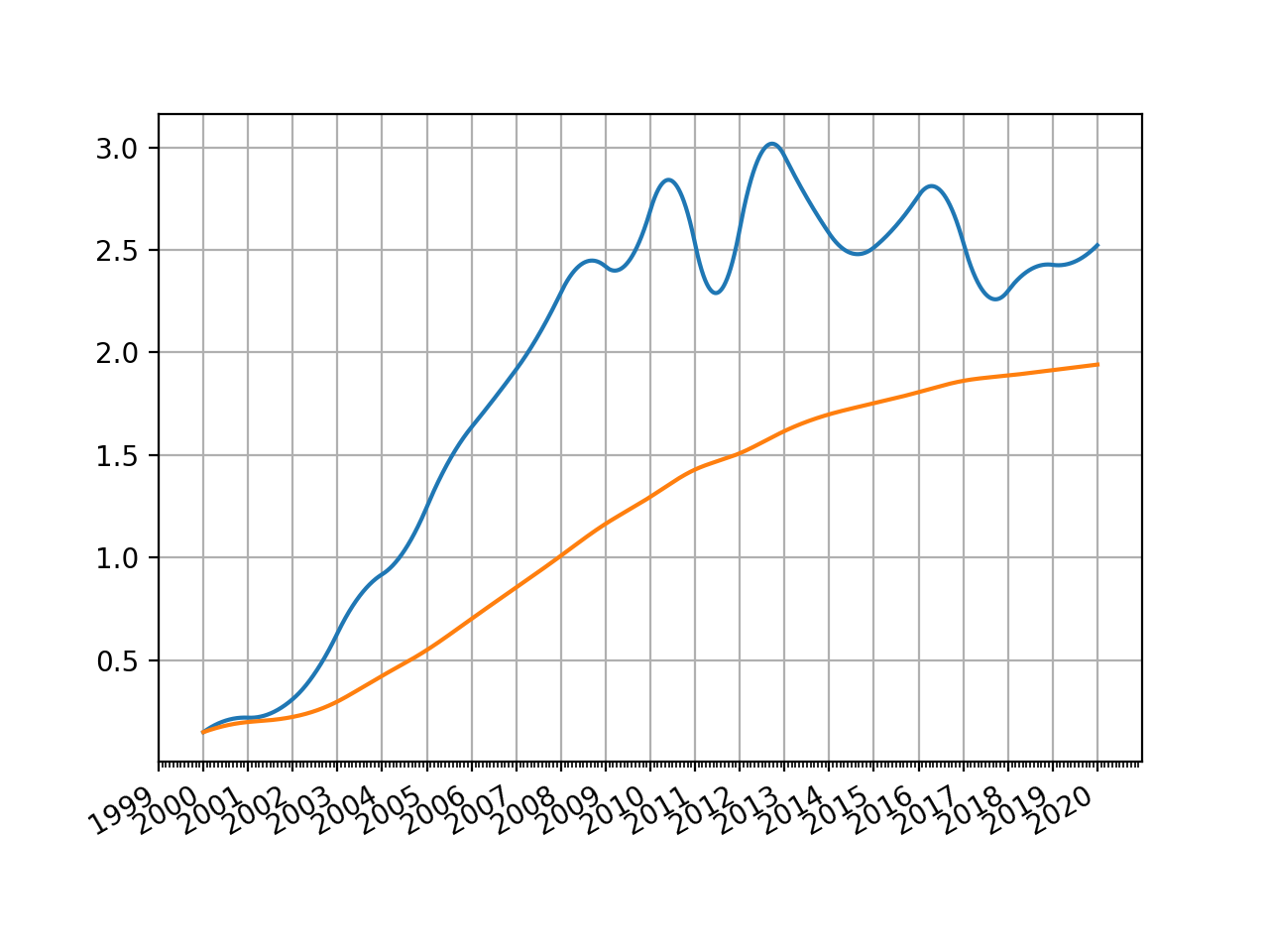
We can plot the resultant curves, which can be compared directly with the EIOPA file.

In [6]: sw.plot("Z")
Out[6]: 
(<Figure size 640x480 with 1 Axes>,
 <Axes: >,
 [<matplotlib.lines.Line2D at 0x1336b6510>])

In [7]: sw.plot("1b")
Out[7]: 
(<Figure size 640x480 with 1 Axes>,
 <Axes: >,
 [<matplotlib.lines.Line2D at 0x1349067b0>])

(Source code, png, hires.png, pdf)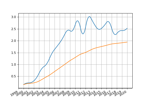

Attributes Summary

ad	Int in {0,1,2} describing the AD order associated with the Curve.
alpha	The \(\alpha\) value of the Curve.
b	The \(\mathbf{\hat{b}}\) parameters value of the Curve.
id	A str identifier to name the Curve used in Solver mappings.
interpolator	An instance of _CurveInterpolator.
k	The \(\kappa\) value as defined in the EIOPA documentation.
meta	An instance of _CurveMeta.
nodes	An instance of _CurveNodes.
u	The \(\mathbf{u}\) vector of the Curve derived from the node dates.
ufr	The UFR value of the Curve.
w	The \(w\) value of the Curve derived from the UFR.

Methods Summary

copy()	Create an identical copy of the curve object.
csolve()	Solves and sets the coefficients, c, of the PPSpline.
index_value(index_date, index_lag[, ...])	Calculate the accrued value of the index from the index_base.
plot(tenor[, right, left, comparators, ...])	Plot given forward tenor rates from the curve.
plot_index([right, left, comparators, ...])	Plot given index values on a Curve.
rate(effective[, termination, modifier, ...])	Calculate the rate on the Curve using DFs.
roll(tenor[, id])	Create a RolledCurve: translating the rate space of Self in time.
shift(spread[, id])	Create a ShiftedCurve: moving Self vertically in rate space.
to_json()	Serialize this object to JSON format.
translate(start[, id])	Create a TranslatedCurve: maintaining an identical rate space, but moving the initial node date forwards in time.
update([nodes])	Update a curves nodes with new, manually input values.
update_meta(key, value)	Update a single meta value on the Curve.
update_node(key, value)	Update a single node value on the Curve.

Attributes Documentation

ad

Int in {0,1,2} describing the AD order associated with the Curve.

alpha

The \(\alpha\) value of the Curve.

b

The \(\mathbf{\hat{b}}\) parameters value of the Curve.

id

A str identifier to name the Curve used in Solver mappings.

interpolator

An instance of _CurveInterpolator.

k

The \(\kappa\) value as defined in the EIOPA documentation.

Under EIOPA:

\[\kappa = \frac{ 1 + \alpha \mathbf{u^T Q b} }{ sinh[\alpha \mathbf{u^T}] \mathbf{Q b} }\]

meta

An instance of _CurveMeta.

nodes

An instance of _CurveNodes.

u

The \(\mathbf{u}\) vector of the Curve derived from the node dates.

ufr

The UFR value of the Curve.

w

The \(w\) value of the Curve derived from the UFR.

Methods Documentation

copy()

Create an identical copy of the curve object.

Return type:

Self

csolve()

Solves and sets the coefficients, c, of the PPSpline.

Return type:

None

Notes

Only impacts curves which have a knot sequence, t, and a PPSpline. Only solves if c not given at curve initialisation.

Uses the spline_endpoints attribute on the class to determine the solving method.

index_value(index_date, index_lag, index_method=IndexMethod.Curve)

Calculate the accrued value of the index from the index_base.

This method will raise if performed on a ‘values’ type Curve.

Parameters:

• index_date (datetime) – The reference date for which the index value will be returned.

• index_lag (int) – The number of months by which to lag the index when determining the value.

• index_method (IndexMethod or str in {"curve", "monthly", "daily"}) – The interpolation method for returning the index value. Monthly returns the index value for the start of the month and daily returns a value based on the interpolation between nodes (which is recommended “linear_index) for InflationCurve.

Return type:

None, float, Dual, Dual2

Notes

The interpolation methods function as follows:

• “curve”: will raise if the requested index_lag does not match the lag attributed to the Curve. In the case the index_lag matches, then the index value for any date is derived via the implied interpolation for the discount factors of the Curve.

  \[I_v(m) = \frac{I_b}{v(m)}\]

• “monthly”: For any date, m, uses the “curve” method having adjusted m in two ways. Firstly it deducts a number of months equal to \(L - L_c\), where L is the given index_lag and \(L_c\) is the index lag of the Curve. And the day of the month is set to 1.

  \[\begin{split}&I^{monthly}_v(m) = I_v(m_adj) \\ &\text{where,} \\ &m_adj = Date(Year(m), Month(m) - L + L_c, 1) \\\end{split}\]

• “daily”: For any date, m, with a given index_lag performs calendar day interpolation on surrounding “monthly” values.

  \[\begin{split}&I^{daily}_v(m) = I^{monthly}_v(m) + \frac{Day(m) - 1}{n} \left ( I^{monthly}_v(m_+) - I^{monthly}_v(m) \right ) \\ &\text{where,} \\ &m_+ = \text{Any date in the month following, }m &n = \text{Calendar days in, } Month(m)\end{split}\]

Examples

The SWESTR rate, for reference value date 6th Sep 2021, was published as 2.375% and the RFR index for that date was 100.73350964. Below we calculate the value that was published for the RFR index on 7th Sep 2021 by the Riksbank.

In [8]: index_curve = Curve(
   ...:     nodes={
   ...:         dt(2021, 9, 6): 1.0,
   ...:         dt(2021, 9, 7): 1 / (1 + 2.375/36000)
   ...:     },
   ...:     index_base=100.73350964,
   ...:     convention="Act360",
   ...:     index_lag=0,
   ...: )
   ...: 

In [9]: index_curve.rate(dt(2021, 9, 6), "1d")
Out[9]: 2.3750000000015703

In [10]: index_curve.index_value(dt(2021, 9, 7), 0)
Out[10]: 100.7401552534832

plot(tenor, right=NoInput.blank, left=NoInput.blank, comparators=NoInput.blank, difference=False, labels=NoInput.blank)

Plot given forward tenor rates from the curve. See notes.

Parameters:

• tenor (str) – The tenor of the forward rates to plot, e.g. “1D”, “3M”.

• right (datetime or str, optional) – The right bound of the graph. If given as str should be a tenor format defining a point measured from the initial node date of the curve. Defaults to the final node of the curve minus the tenor.

• left (datetime or str, optional) – The left bound of the graph. If given as str should be a tenor format defining a point measured from the initial node date of the curve. Defaults to the initial node of the curve.

• comparators (list[Curve]) – A list of curves which to include on the same plot as comparators.

• difference (bool) – Whether to plot as comparator minus base curve or outright curve levels in plot. Default is False.

• labels (list[str]) – A list of strings associated with the plot and comparators. Must be same length as number of plots.

Returns:

(fig, ax, line)

Return type:

Matplotlib.Figure, Matplotplib.Axes, Matplotlib.Lines2D

Notes

This function plots single-period, simple interest curve rates, which are defined as:

\[1 + r d = \frac{v_{start}}{v_{end}}\]

where d is the day count fraction determined using the convention associated with the Curve.

This function does not plot swap rates, which is impossible since the Curve object contains no information regarding the parameters of the ‘swap’ (e.g. its frequency or its convention etc.). If tenors longer than one year are sought results may start to deviate from those one might expect. See Issue 246.

plot_index(right=NoInput.blank, left=NoInput.blank, comparators=NoInput.blank, difference=False, labels=NoInput.blank, interpolation='curve')

Plot given index values on a Curve.

Parameters:

• right (datetime or str, optional) – The right bound of the graph. If given as str should be a tenor format defining a point measured from the initial node date of the curve. Defaults to the final node of the curve minus the tenor.

• left (datetime or str, optional) – The left bound of the graph. If given as str should be a tenor format defining a point measured from the initial node date of the curve. Defaults to the initial node of the curve.

• comparators (list[Curve]) – A list of curves which to include on the same plot as comparators.

• difference (bool) – Whether to plot as comparator minus base curve or outright curve levels in plot. Default is False.

• labels (list[str]) – A list of strings associated with the plot and comparators. Must be same length as number of plots.

• interpolation (str in {"curve", "daily", "monthly"}) – The type of index interpolation method to use.

Returns:

(fig, ax, line)

Return type:

Matplotlib.Figure, Matplotplib.Axes, Matplotlib.Lines2D

rate(effective, termination=NoInput.blank, modifier=NoInput.inherit, float_spread=NoInput.blank, spread_compound_method=NoInput.blank)

Calculate the rate on the Curve using DFs.

If rates are sought for dates prior to the initial node of the curve None will be returned.

Parameters:

• effective (datetime) – The start date of the period for which to calculate the rate.

• termination (datetime or str) – The end date of the period for which to calculate the rate.

• modifier (str, optional) – The day rule if determining the termination from tenor. If False is determined from the Curve modifier.

• float_spread (float, optional) – A float spread can be added to the rate in certain cases.

• spread_compound_method (str in {"none_simple", "isda_compounding"}) – The method if adding a float spread. If “none_simple” is used this results in an exact calculation. If “isda_compounding” or “isda_flat_compounding” is used this results in an approximation.

Return type:

Dual, Dual2 or float

Notes

Calculating rates from a curve implies that the conventions attached to the specific index, e.g. USD SOFR, or GBP SONIA, are applicable and these should be set at initialisation of the Curve. Thus, the convention used to calculate the rate is taken from the Curve from which rate is called.

modifier is only used if a tenor is given as the termination.

Major indexes, such as legacy IBORs, and modern RFRs typically use a convention which is either “Act365F” or “Act360”. These conventions do not need additional parameters, such as the termination of a leg, the frequency or a leg or whether it is a stub to calculate a DCF.

Adding Floating Spreads

An optimised method for adding floating spreads to a curve rate is provided. This is quite restrictive and mainly used internally to facilitate other parts of the library.

• When spread_compound_method is “none_simple” the spread is a simple linear addition.

• When using “isda_compounding” or “isda_flat_compounding” the curve is assumed to be comprised of RFR rates and an approximation is used to derive to total rate.

Examples

In [11]: curve_act365f = Curve(
   ....:     nodes={
   ....:         dt(2022, 1, 1): 1.0,
   ....:         dt(2022, 2, 1): 0.98,
   ....:         dt(2022, 3, 1): 0.978,
   ....:     },
   ....:     convention='Act365F'
   ....: )
   ....: 

In [12]: curve_act365f.rate(dt(2022, 2, 1), dt(2022, 3, 1))
Out[12]: 2.6657902424774402

Using a different convention will result in a different rate:

In [13]: curve_act360 = Curve(
   ....:     nodes={
   ....:         dt(2022, 1, 1): 1.0,
   ....:         dt(2022, 2, 1): 0.98,
   ....:         dt(2022, 3, 1): 0.978,
   ....:     },
   ....:     convention='Act360'
   ....: )
   ....: 

In [14]: curve_act360.rate(dt(2022, 2, 1), dt(2022, 3, 1))
Out[14]: 2.6292725679229547

roll(tenor, id=NoInput.blank)

Create a RolledCurve: translating the rate space of Self in time.

For examples see the documentation for RolledCurve.

Parameters:

• tenor (datetime, str or int) – The measure of time by which to translate the curve through time.

• id (str, optional) – Set the id of the returned curve.

Return type:

RolledCurve

shift(spread, id=NoInput.blank)

Create a ShiftedCurve: moving Self vertically in rate space.

For examples see the documentation for ShiftedCurve.

Parameters:

• spread (float, Dual, Dual2, Variable) – The number of basis points added to the existing curve.

• id (str, optional) – Set the id of the returned curve.

Return type:

ShiftedCurve

to_json()

Serialize this object to JSON format.

The object can be deserialized using the from_json() method.

Return type:

str

Notes

Some Curves will not be serializable, for example those that possess user defined interpolation functions.

translate(start, id=NoInput.blank)

Create a TranslatedCurve: maintaining an identical rate space, but moving the initial node date forwards in time.

For examples see the documentation for TranslatedCurve.

Parameters:

• start (datetime) – The new initial node date for the curve. Must be after the original initial node date.

• id (str, optional) – Set the id of the returned curve.

Return type:

TranslatedCurve

update(nodes=NoInput.blank)

Update a curves nodes with new, manually input values.

For arguments see Curve. Any value not given will not change the underlying Curve.

Parameters:

nodes (dict[datetime, DualTypes], optional) – New nodes to assign to the curve.

Return type:

None

Notes

Warning

Rateslib is an object-oriented library that uses complex associations. Although Python may not object to directly mutating attributes of a Curve instance, this should be avoided in rateslib. Only use official update methods to mutate the values of an existing Curve instance. This class is labelled as a mutable on update object.

update_meta(key, value)

Update a single meta value on the Curve.

Parameters:

• key (datetime) – The meta descriptor to update. Must be a documented attribute of _CurveMeta.

• value (Any) – Value to update on the Curve.

Return type:

None

update_node(key, value)

Update a single node value on the Curve.

Parameters:

• key (datetime) – The node date to update. Must exist in nodes.

• value (float, Dual, Dual2, Variable) – Value to update on the Curve.

Return type:

None

Notes

Warning

Rateslib is an object-oriented library that uses complex associations. Although Python may not object to directly mutating attributes of a Curve instance, this should be avoided in rateslib. Only use official update methods to mutate the values of an existing Curve instance. This class is labelled as a mutable on update object.