
User Guide#
Where to start?#
Rateslib tends to follow the typical quant architecture:
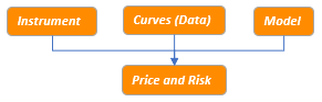
This means that financial instrument specification, curve and/or surface construction from market data including foreign exchange (FX) will permit pricing metrics and risk sensitivity. These functionalities are interlinked and potentially dependent upon each other. This guide will introduce them in a structured way and give typical examples how they are used in practice.
Let’s start with some fundamental Curve and Instrument constructors.
Trivial derivatives examples#
Rateslib has two fundamental Curve types. Most of the time you
will only need to use a Curve.
A Curve is discount factor (DF) based and is constructed
by providing DFs on specific node dates. Interpolation between nodes is
configurable, but the below uses the “log-linear” default.
In [1]: from rateslib import *

In [2]: usd_curve = Curve(
   ...:     nodes={
   ...:         dt(2022, 1, 1): 1.0,
   ...:         dt(2022, 7, 1): 0.98,
   ...:         dt(2023, 1, 1): 0.95
   ...:     },
   ...:     calendar="nyc",
   ...:     id="sofr",
   ...: )
   ...:
A LineCurve is value based and is constructed
by providing curve values on specific node dates. Interpolation between nodes is
configurable, with the default being “linear” interpolation (hence LineCurve). This type
has no DFs so can’t be used for discounting cashflows.
In [3]: usd_legacy_3mIBOR = LineCurve(
   ...:     nodes={
   ...:         dt(2022, 1, 1): 2.635,
   ...:         dt(2022, 7, 1): 2.896,
   ...:         dt(2023, 1, 1): 2.989,
   ...:     },
   ...:     calendar="nyc",
   ...:     id="us_ibor_3m",
   ...: )
   ...:
An Index Curve is required by certain products, e.g.
inflation linked bonds (IndexFixedRateBond) or
zero coupon inflation swaps (ZCIS). Adding index_base
and index_lag argument inputs extends a DF based Curve to
work in these cases.
In [4]: usd_cpi = Curve(
   ...:     nodes={
   ...:         dt(2022, 1, 1): 1.00,
   ...:         dt(2022, 7, 1): 0.97,
   ...:         dt(2023, 1, 1): 0.955,
   ...:     },
   ...:     index_base=308.95,
   ...:     index_lag=3,
   ...:     interpolation="linear_index",
   ...:     id="us_cpi",
   ...: )
   ...:
A Hazard Curve is used by credit Instruments when a default is possible. Hazard Curves
utilise the same Curve class and the rates reflect overnight
hazard rates and the DFs reflect survival probabilities.
In [5]: pfizer_hazard = Curve(
   ...:     nodes={
   ...:         dt(2022, 1, 1): 1.0,
   ...:         dt(2022, 7, 1): 0.998,
   ...:         dt(2023, 1, 1): 0.995
   ...:     },
   ...:     id="pfizer_hazard",
   ...:     credit_recovery_rate=0.4,
   ...:     credit_discretization=23,
   ...: )
   ...:
Next, we will construct some basic derivative Instruments. These will use some market conventions defined by rateslib through its default argument specifications, although all arguments can be supplied manually if and when required.
Here we create a short dated SOFR RFR interest rate swap (IRS).
In [6]: irs = IRS(
   ...:     effective=dt(2022, 2, 15),
   ...:     termination="6m",
   ...:     notional=1000000000,
   ...:     fixed_rate=2.0,
   ...:     spec="usd_irs"
   ...: )
   ...:
Here we create a SOFR STIR future (STIRFuture).
In [7]: stir = STIRFuture(
   ...:     effective=get_imm(code="H22"),
   ...:     termination=get_imm(code="M22"),
   ...:     contracts=100,
   ...:     price=97.495,
   ...:     spec="usd_stir",
   ...: )
   ...:
A US LIBOR FRA is an obsolete Instrument, but we can still
create one and these still trade in other currencies, e.g. EUR.
In [8]: fra = FRA(
   ...:     effective=dt(2022, 2, 16),
   ...:     termination="3m",
   ...:     frequency="Q",
   ...:     calendar="nyc",
   ...:     convention="act360",
   ...:     leg2_method_param=2,
   ...:     fixed_rate=2.5
   ...: )
   ...:
Here we construct a generic US investment grade credit default
swap (CDS)
In [9]: cds = CDS(
   ...:     effective=dt(2021, 12, 20),
   ...:     termination=dt(2022, 9, 20),
   ...:     notional=15e6,
   ...:     spec="us_ig_cds",
   ...: )
   ...:
This constructs a zero-coupon inflation swap
(ZCIS) with usual
daily index interpolation and 3-month index lag.
In [10]: zcis = ZCIS(
   ....:     effective=dt(2022, 2, 2),
   ....:     termination="9m",
   ....:     notional=-25e6,
   ....:     fixed_rate=3.25,
   ....:     spec="usd_zcis",
   ....: )
   ....:
We can combine the Curves and the Instruments to give pricing metrics such as
npv(),
cashflows(), and the mid-market
rate(), as well as others. Without further specification
these values are all expressed in the Instrument’s local USD settlement currency.
In [11]: irs.npv(curves=usd_curve)
Out[11]: 12629097.829705866
In [12]: irs.cashflows(curves=usd_curve)
Out[12]:
               Type  Ccy    Payment       Notional Period Convention  DCF  Acc Start    Acc End   DF     Cashflow         NPV  FX Rate Base Ccy     NPV Ccy Collateral  Rate  Spread
leg1 0  FixedPeriod  USD 2022-08-17  1000000000.00   Stub     Act360 0.50 2022-02-15 2022-08-15 0.97 -10055555.56 -9776494.15     1.00      USD -9776494.15       None  2.00     NaN
leg2 0  FloatPeriod  USD 2022-08-17 -1000000000.00   Stub     Act360 0.50 2022-02-15 2022-08-15 0.97  23045139.84 22405591.98     1.00      USD 22405591.98       None  4.58    0.00
In [13]: stir.npv(curves=usd_curve)
Out[13]: -383423.5359790483
In [14]: stir.rate(curves=usd_curve, metric="price")
Out[14]: 95.96130585608381
In [15]: fra.npv(curves=[usd_legacy_3mIBOR, usd_curve])
Out[15]: 484.85927030340326
In [16]: fra.rate(curves=[usd_legacy_3mIBOR, usd_curve])
Out[16]: 2.698447513812155
In [17]: cds.npv(curves=[pfizer_hazard, usd_curve])
Out[17]: -82285.89860611843
In [18]: cds.rate(curves=[pfizer_hazard, usd_curve])
Out[18]: 0.26322526465564466
In [19]: cds.cashflows(curves=[pfizer_hazard, usd_curve])
Out[19]:
                          Type  Ccy    Payment     Notional   Period Convention  DCF  Acc Start    Acc End  Rate Spread   DF   Cashflow       NPV  FX Rate Base Ccy   NPV Ccy Collateral  Survival  Recovery
leg1 0     CreditPremiumPeriod  USD 2022-03-21  15000000.00  Regular     Act360 0.25 2021-12-20 2022-03-21  1.00   None 0.99  -37916.67 -37569.55     1.00      USD -37569.55       None      1.00      0.40
     1     CreditPremiumPeriod  USD 2022-06-21  15000000.00  Regular     Act360 0.26 2022-03-21 2022-06-21  1.00   None 0.98  -38333.33 -37556.66     1.00      USD -37556.66       None      1.00      0.40
     2     CreditPremiumPeriod  USD 2022-09-20  15000000.00  Regular     Act360 0.25 2022-06-21 2022-09-20  1.00   None 0.97  -37916.67 -36557.72     1.00      USD -36557.72       None      1.00      0.40
leg2 0  CreditProtectionPeriod  USD 2022-09-20 -15000000.00     Stub     Act360 0.76 2021-12-20 2022-09-20   NaN    NaN 0.97 9000000.00  29398.03     1.00      USD  29398.03       None      1.00      0.40
In [20]: zcis.npv(curves=[usd_cpi, usd_curve])
Out[20]: -285438.4728524148
In [21]: zcis.rate(curves=[usd_cpi, usd_curve])
Out[21]: 4.852119618886386
In [22]: zcis.cashflows(curves=[usd_cpi, usd_curve])
Out[22]:
                   Type  Ccy    Payment     Notional Period   Convention  DCF  Acc Start    Acc End   DF   Cashflow        NPV  FX Rate Base Ccy    NPV Ccy Collateral  Rate Spread  Index Base  Index Val  Index Ratio Index Fix Date  Unindexed Cashflow
leg1 0  ZeroFixedPeriod  USD 2022-11-02 -25000000.00   Stub  YearsMonths 0.75 2022-02-02 2022-11-02 0.96  606932.34  582461.01     1.00      USD  582461.01       None  3.25   None         NaN        NaN          NaN            NaT                 NaN
leg2 0         Cashflow  USD 2022-11-02  25000000.00    NaN          NaN  NaN        NaT        NaT 0.96 -904363.13 -867899.49     1.00      USD -867899.49       None   NaN    NaN      310.64     321.88         1.04     2022-11-02        -25000000.00
Securities and bonds#
Rateslib is steadily building a collection of market conventions for a host of global bonds. Again these specifications are available at default argument specifications for those that have already been populated.
A very common instrument in financial investing is a FixedRateBond.
At time of writing the on-the-run 10Y US treasury was the 3.875% Aug 2033 bond. Here we
construct this using the street convention and derive the price from yield-to-maturity and
risk calculations.
In [23]: fxb = FixedRateBond(
   ....:     effective=dt(2023, 8, 15),
   ....:     termination=dt(2033, 8, 15),
   ....:     fixed_rate=3.875,
   ....:     spec="us_gb"  # US Government Bond
   ....: )
   ....:

In [24]: fxb.accrued(settlement=dt(2025, 2, 14))
Out[24]: 1.9269701086956519

In [25]: fxb.price(ytm=4.0, settlement=dt(2025, 2, 14))
Out[25]: 99.10641380057267

In [26]: fxb.duration(ytm=4.0, settlement=dt(2025, 2, 14), metric="duration")
Out[26]: np.float64(7.178560455252011)

In [27]: fxb.duration(ytm=4.0, settlement=dt(2025, 2, 14), metric="modified")
Out[27]: np.float64(7.037804367894129)

In [28]: fxb.duration(ytm=4.0, settlement=dt(2025, 2, 14), metric="risk")
Out[28]: np.float64(7.11053190579773)
A FloatRateNote can also be constructed. The below bond
settles to 3M-TermSOFR which is an IBOR style term fixing_method (and we simulate
its pricing with the Curves already constructed). Compounded RFR
FRNs can also be constructed, using other method inputs.
In [29]: frn = FloatRateNote(
   ....:     effective=dt(2021, 8, 15),
   ....:     termination=dt(2022, 8, 15),
   ....:     frequency="Q",
   ....:     float_spread=86.0,
   ....:     spread_compound_method="none_simple",
   ....:     convention="act360",
   ....:     calendar="nyc",
   ....:     payment_lag=0,
   ....:     fixing_method="ibor",
   ....:     method_param=0,  # fixing lag is 0 business days
   ....:     rate_fixings=[2.00, 2.14],
   ....:     ex_div=1,
   ....:     settle=1,
   ....:     currency="usd",
   ....: )
   ....:

In [30]: frn.accrued(settlement=dt(2022, 1, 2))
Out[30]: 0.3999999999999999

In [31]: frn.rate(curves=[usd_legacy_3mIBOR, usd_curve])
Out[31]: 99.41819186149803

In [32]: frn.cashflows(curves=[usd_legacy_3mIBOR, usd_curve])
Out[32]:
               Type  Ccy    Payment   Notional   Period Convention  DCF  Acc Start    Acc End   DF    Cashflow        NPV  FX Rate Base Ccy    NPV Ccy Collateral  Rate  Spread
leg1 0  FloatPeriod  USD 2021-11-15 1000000.00  Regular     Act360 0.25 2021-08-16 2021-11-15 0.00    -7229.44       0.00     1.00      USD       0.00       None  2.86   86.00
     1  FloatPeriod  USD 2022-02-15 1000000.00  Regular     Act360 0.26 2021-11-15 2022-02-15 0.99    -7666.67   -7628.26     1.00      USD   -7628.26       None  3.00   86.00
     2  FloatPeriod  USD 2022-05-16 1000000.00  Regular     Act360 0.25 2022-02-15 2022-05-16 0.99    -8899.72   -8766.63     1.00      USD   -8766.63       None  3.56   86.00
     3  FloatPeriod  USD 2022-08-15 1000000.00  Regular     Act360 0.25 2022-05-16 2022-08-15 0.97    -9326.66   -9070.89     1.00      USD   -9070.89       None  3.69   86.00
     4     Cashflow  USD 2022-08-15 1000000.00      NaN        NaN  NaN        NaT        NaT 0.97 -1000000.00 -972576.66     1.00      USD -972576.66       None   NaN     NaN
Below we construct a US government bond Bill using
default spec.
In [33]: bill = Bill(
   ....:     effective=dt(2024, 10, 24),
   ....:     termination=dt(2025, 4, 24),
   ....:     spec="us_gbb",  # US Government Bond-Bill
   ....: )
   ....:

In [34]: bill.discount_rate(price=99.0808021, settlement=dt(2025, 2, 4))
Out[34]: 4.188749924050641

In [35]: bill.ytm(price=99.0808021, settlement=dt(2025, 2, 4))
Out[35]: 4.300459677867501

In [36]: bill.duration(ytm=4.18875, settlement=dt(2025, 2, 4), metric="risk")
Out[36]: np.float64(0.21944444444444444)

In [37]: bill.price(rate=4.18875, settlement=dt(2025, 2, 4))
Out[37]: 99.08080208333334
Below we construct an IndexFixedRateBond, using relevant
indexing arguments.
In [38]: ifrb = IndexFixedRateBond(  # CUSIP:91282CCA7 ISIN:US91282CCA71
   ....:     effective=dt(2021, 4, 15),
   ....:     termination=dt(2026, 4, 15),
   ....:     fixed_rate=0.125,
   ....:     index_base=262.250270,
   ....:     index_fixings=265.0,
   ....:     spec="us_gbi",
   ....: )
   ....:

In [39]: ifrb.price(ytm=1.397926, settlement=dt(2025, 2, 4))
Out[39]: 98.49999982402322

In [40]: ifrb.accrued(settlement=dt(2025, 2, 4))
Out[40]: 0.038461538461538464

In [41]: ifrb.cashflows(curves=[usd_cpi, usd_curve])
Out[41]:
                Type  Ccy    Payment   Notional   Period  Convention  DCF  Acc Start    Acc End   DF    Cashflow         NPV  FX Rate Base Ccy     NPV Ccy Collateral  Rate  Spread  Index Base  Index Val  Index Ratio Index Fix Date  Unindexed Cashflow
leg1 0   FixedPeriod  USD 2021-10-15 1000000.00  Regular  ActActICMA 0.50 2021-04-15 2021-10-15 0.00     -631.55        0.00     1.00      USD        0.00       None  0.12     NaN      262.25     265.00         1.01     2021-10-15             -625.00
     1   FixedPeriod  USD 2022-04-18 1000000.00  Regular  ActActICMA 0.50 2021-10-15 2022-04-15 0.99     -749.38     -740.48     1.00      USD     -740.48       None  0.12     NaN      262.25     314.44         1.20     2022-04-15             -625.00
     2   FixedPeriod  USD 2022-10-17 1000000.00  Regular  ActActICMA 0.50 2022-04-15 2022-10-15 0.96     -765.94     -737.04     1.00      USD     -737.04       None  0.12     NaN      262.25     321.39         1.23     2022-10-15             -625.00
     3   FixedPeriod  USD 2023-04-17 1000000.00  Regular  ActActICMA 0.50 2022-10-15 2023-04-15 0.93     -777.73     -725.73     1.00      USD     -725.73       None  0.12     NaN      262.25     326.34         1.24     2023-04-15             -625.00
     4   FixedPeriod  USD 2023-10-16 1000000.00  Regular  ActActICMA 0.50 2023-04-15 2023-10-15 0.90     -789.59     -714.48     1.00      USD     -714.48       None  0.12     NaN      262.25     331.31         1.26     2023-10-15             -625.00
     5   FixedPeriod  USD 2024-04-15 1000000.00  Regular  ActActICMA 0.50 2023-10-15 2024-04-15 0.88     -801.44     -703.25     1.00      USD     -703.25       None  0.12     NaN      262.25     336.29         1.28     2024-04-15             -625.00
     6   FixedPeriod  USD 2024-10-15 1000000.00  Regular  ActActICMA 0.50 2024-04-15 2024-10-15 0.85     -813.30     -691.92     1.00      USD     -691.92       None  0.12     NaN      262.25     341.26         1.30     2024-10-15             -625.00
     7   FixedPeriod  USD 2025-04-15 1000000.00  Regular  ActActICMA 0.50 2024-10-15 2025-04-15 0.82     -825.10     -680.70     1.00      USD     -680.70       None  0.12     NaN      262.25     346.21         1.32     2025-04-15             -625.00
     8   FixedPeriod  USD 2025-10-15 1000000.00  Regular  ActActICMA 0.50 2025-04-15 2025-10-15 0.80     -836.95     -669.45     1.00      USD     -669.45       None  0.12     NaN      262.25     351.19         1.34     2025-10-15             -625.00
     9   FixedPeriod  USD 2026-04-15 1000000.00  Regular  ActActICMA 0.50 2025-10-15 2026-04-15 0.78     -848.75     -658.33     1.00      USD     -658.33       None  0.12     NaN      262.25     356.13         1.36     2026-04-15             -625.00
     10     Cashflow  USD 2026-04-15 1000000.00      NaN         NaN  NaN        NaT        NaT 0.78 -1357993.45 -1053323.30     1.00      USD -1053323.30       None   NaN     NaN      262.25     356.13         1.36     2026-04-15         -1000000.00
There are some interesting Cookbook articles
on BondFuture and cheapest-to-deliver (CTD) analysis.
Quick look at FX#
Spot rates and conversion#
The above values were all calculated and displayed in USD. That is the default
currency in rateslib and the local currency of those Instruments. We can convert these values
into another currency using the FXRates class. This is a basic class which is
parametrised by some exchange rates.
In [42]: fxr = FXRates({"eurusd": 1.05, "gbpusd": 1.25})

In [43]: fxr.rates_table()
Out[43]:
     usd  eur  gbp
usd 1.00 0.95 0.80
eur 1.05 1.00 0.84
gbp 1.25 1.19 1.00
We now have a mechanism by which to specify values in other currencies.
In [44]: irs.npv(curves=usd_curve, fx=fxr, base="usd")
Out[44]: 12629097.829705866

In [45]: irs.npv(curves=usd_curve, fx=fxr, base="eur")
Out[45]: <Dual: 12027712.218767, (fx_eurusd), [-11454964.0]>
In [46]: stir.npv(curves=usd_curve, fx=fxr, base="usd")
Out[46]: -383423.5359790483

In [47]: stir.npv(curves=usd_curve, fx=fxr, base="eur")
Out[47]: <Dual: -365165.272361, (fx_eurusd), [347776.4]>
In [48]: fra.npv(curves=[usd_legacy_3mIBOR, usd_curve], fx=fxr, base="usd")
Out[48]: 484.85927030340326

In [49]: fra.npv(curves=[usd_legacy_3mIBOR, usd_curve], fx=fxr, base="eur")
Out[49]: <Dual: 461.770734, (fx_eurusd), [-439.8]>
In [50]: cds.npv(curves=[pfizer_hazard, usd_curve], fx=fxr, base="usd")
Out[50]: -82285.89860611843

In [51]: cds.npv(curves=[pfizer_hazard, usd_curve], fx=fxr, base="eur")
Out[51]: <Dual: -78367.522482, (fx_eurusd), [74635.7]>
In [52]: zcis.npv(curves=[usd_cpi, usd_curve], fx=fxr, base="usd")
Out[52]: -285438.4728524148

In [53]: zcis.npv(curves=[usd_cpi, usd_curve], fx=fxr, base="eur")
Out[53]: <Dual: -271846.164621, (fx_eurusd), [258901.1]>
One observes that the value returned here is not a float but a Dual
which is part of rateslib’s AD framework. This is the first example of capturing a
sensitivity, which here denotes the sensitivity of the EUR NPV relative to the EURUSD FX rate.
One can read more about this particular treatment of FX
here and more generally about the dual AD framework here.
FX forwards#
For multi-currency derivatives we need more than basic, spot exchange rates.
We need an FXForwards market.
This stores the FX rates and the interest
rates curves that are used for all the FX-interest rate parity derivations. With these
we can calculate forward FX rates and also ad-hoc FX swap rates.
When defining the fx_curves dict mapping, the key “eurusd” should be interpreted as; the
Curve for EUR cashflows, collateralised in USD, and similarly for other entries.
In [54]: eur_curve = Curve({
   ....:     dt(2022, 1, 1): 1.0,
   ....:     dt(2022, 7, 1): 0.972,
   ....:     dt(2023, 1, 1): 0.98},
   ....:     calendar="tgt",
   ....: )
   ....:

In [55]: eurusd_curve = Curve({
   ....:     dt(2022, 1, 1): 1.0,
   ....:     dt(2022, 7, 1): 0.973,
   ....:     dt(2023, 1, 1): 0.981}
   ....: )
   ....:

In [56]: fxf = FXForwards(
   ....:     fx_rates=FXRates({"eurusd": 1.05}, settlement=dt(2022, 1, 1)),
   ....:     fx_curves={
   ....:         "usdusd": usd_curve,
   ....:         "eureur": eur_curve,
   ....:         "eurusd": eurusd_curve,
   ....:     }
   ....: )
   ....:

In [57]: fxf.rate("eurusd", settlement=dt(2023, 1, 1))
Out[57]: <Dual: 1.084263, (fx_eurusd), [1.0]>

In [58]: fxf.swap("eurusd", settlements=[dt(2022, 2, 1), dt(2022, 5, 2)])
Out[58]: <Dual: -37.314180, (fx_eurusd), [-35.5]>
FXForwards objects are comprehensive and more information regarding all of the FX features is available in this link.
More about instruments#
We’ve seen some single currency derivatives above. A complete guide for all of the Instruments is available in this link. That will also introduce the building blocks; Legs and Periods.
Multi-currency instruments#
Let’s take a look at the multi-currency instruments. Notice how these Instruments
maintain consistent method naming conventions with those above. This makes it possible to plug
any Instruments into a Solver to calibrate Curves
around target mid-market rates, and generate market risks.
This is an FXSwap.
In [59]: fxs = FXSwap(
   ....:     effective=dt(2022, 2, 1),
   ....:     termination="3m",  # May-1 is a holiday, May-2 is business end date.
   ....:     pair="eurusd",
   ....:     notional=20e6,
   ....:     calendar="tgt|fed",
   ....: )
   ....:

In [60]: fxs.rate(curves=[eurusd_curve, usd_curve], fx=fxf)
Out[60]: <Dual: -37.314180, (fx_eurusd), [-35.5]>

In [61]: fxs.cashflows_table(curves=[eurusd_curve, usd_curve], fx=fxf)
Out[61]:
local_ccy               EUR          USD
collateral_ccy          usd          usd
payment
2022-02-01     -20000000.00  20974233.02
2022-05-02      20000000.00 -20899604.66
An FXForward is a forward FX transaction.
In [62]: fxe = FXForward(
   ....:     settlement=dt(2022, 4, 1),
   ....:     pair="eurusd",
   ....:     notional=10e6,
   ....:     fx_rate=1.035,
   ....: )
   ....:

In [63]: fxe.rate(curves=[eurusd_curve, usd_curve], fx=fxf)
Out[63]: <Dual: 1.046264, (fx_eurusd), [1.0]>

In [64]: fxe.npv(curves=[eurusd_curve, usd_curve], fx=fxf)
Out[64]: <Dual: 106203.917957, (fx_eurusd), [9293922.1]>

In [65]: fxe.cashflows_table(curves=[eurusd_curve, usd_curve], fx=fxf)
Out[65]:
local_ccy              EUR          USD
collateral_ccy         usd          usd
payment
2022-04-01     10000000.00 -10350000.00
Cross-currency swaps (XCS) are easily configured and
analysed in rateslib.
In [66]: xcs = XCS(
   ....:     effective=dt(2022, 4, 1),
   ....:     termination="6m",
   ....:     spec="eurusd_xcs",
   ....:     float_spread=-3.0,
   ....:     notional=25e6,
   ....: )
   ....:

In [67]: xcs.rate(curves=[eur_curve, eurusd_curve, usd_curve, usd_curve], fx=fxf)
Out[67]: <Dual: -10.421943, (fx_eurusd), [-0.0]>

In [68]: xcs.cashflows(curves=[eur_curve, eurusd_curve, usd_curve, usd_curve], fx=fxf)
Out[68]:
               Type  Ccy    Payment     Notional   DF     Cashflow          NPV  FX Rate Base Ccy      NPV Ccy Collateral   Period Convention  DCF  Acc Start    Acc End  Rate  Spread  FX Fixing FX Fix Date Reference Ccy
leg1 0     Cashflow  EUR 2022-04-01 -25000000.00 0.99  25000000.00  24662055.24     1.00      EUR  24662055.24        usd      NaN        NaN  NaN        NaT        NaT   NaN     NaN        NaN         NaT           NaN
     1  FloatPeriod  EUR 2022-07-06  25000000.00 0.97   -357619.39   -348041.10     1.00      EUR   -348041.10        usd  Regular     Act360 0.25 2022-04-01 2022-07-01  5.66   -3.00        NaN         NaT           NaN
     2  FloatPeriod  EUR 2022-10-05  25000000.00 0.98    106426.42    103996.26     1.00      EUR    103996.26        usd  Regular     Act360 0.26 2022-07-01 2022-10-03 -1.63   -3.00        NaN         NaT           NaN
     3     Cashflow  EUR 2022-10-03  25000000.00 0.98 -25000000.00 -24426969.29     1.00      EUR -24426969.29        usd      NaN        NaN  NaN        NaT        NaT   NaN     NaN        NaN         NaT           NaN
leg2 0     Cashflow  USD 2022-04-01  25000000.00 0.99 -26156599.95 -25895158.01     1.00      USD -25895158.01        usd      NaN        NaN  NaN        NaT        NaT   NaN     NaN       1.05  2022-03-30           EUR
     1  FloatPeriod  USD 2022-07-06 -25000000.00 0.98    267030.67    261469.06     1.00      USD    261469.06        usd  Regular     Act360 0.25 2022-04-01 2022-07-01  4.04    0.00       1.05  2022-03-30           EUR
     2  MtmCashflow  USD 2022-07-01  25000000.00 0.98     94099.95     92217.95     1.00      USD     92217.95        usd      NaN        NaN  NaN        NaT        NaT   NaN     NaN       1.04  2022-06-29           EUR
     3  FloatPeriod  USD 2022-10-05 -25000000.00 0.96    417261.77    402336.93     1.00      USD    402336.93        usd  Regular     Act360 0.26 2022-07-01 2022-10-03  6.13    0.00       1.04  2022-06-29           EUR
     4     Cashflow  USD 2022-10-03 -25000000.00 0.96  26062500.00  25138777.08     1.00      USD  25138777.08        usd      NaN        NaN  NaN        NaT        NaT   NaN     NaN       1.04  2022-06-29           EUR

In [69]: xcs.cashflows_table(curves=[eur_curve, eurusd_curve, usd_curve, usd_curve], fx=fxf)
Out[69]:
local_ccy               EUR          USD
collateral_ccy          usd          usd
payment
2022-04-01      25000000.00 -26156599.95
2022-07-01             0.00     94099.95
2022-07-06       -357619.39    267030.67
2022-10-03     -25000000.00  26062500.00
2022-10-05        106426.42    417261.77
Non-deliverable forwards (NDF) can be constructed.
In [70]: ndf = NDF(
   ....:     settlement=dt(2022, 8, 15),
   ....:     pair="eurusd",
   ....:     notional=10e6,  # 10mm EUR
   ....:     fx_rate=1.1
   ....: )
   ....:

In [71]: ndf.rate(fx=fxf)
Out[71]: <Dual: 1.052563, (fx_eurusd), [1.0]>

In [72]: ndf.cashflows(curves=usd_curve, fx=fxf)
Out[72]:
            Type  Ccy    Payment     Notional   DF     Cashflow          NPV  FX Rate Base Ccy      NPV Ccy Collateral  FX Fixing FX Fix Date Reference Ccy
leg1 0  Cashflow  EUR 2022-08-15 -10000000.00 0.97  10000000.00   9725766.55     1.00      EUR   9725766.55        usd        NaN         NaT           NaN
leg2 0  Cashflow  EUR 2022-08-15  11000000.00 0.97 -10450682.94 -10164090.26     1.00      EUR -10164090.26        usd       1.05  2022-08-11           USD

In [73]: ndf.cashflows_table(curves=usd_curve, fx=fxf)
Out[73]:
local_ccy             EUR
collateral_ccy        usd
payment
2022-08-15     -450682.94
A Non-deliverable IRS (IRS) can be constructed.
In [74]: ndirs = IRS(
   ....:     currency="usd",   #  <- local settlement currency
   ....:     pair="eurusd",    #  <- EUR is the reference and notional currency
   ....:     effective=dt(2022, 2, 1),
   ....:     termination="2M",
   ....:     frequency="M",
   ....:     notional=10e6,    # 10mm EUR
   ....:     calendar="tgt|fed",
   ....: )
   ....:

In [75]: ndirs.rate(curves=[eur_curve, usd_curve], fx=fxf)
Out[75]: <Dual: 5.661639, (fx_eurusd), [0.0]>

In [76]: ndirs.cashflows(curves=[eur_curve, usd_curve], fx=fxf)
Out[76]:
               Type  Ccy    Payment     Notional   Period Convention  DCF  Acc Start    Acc End   DF  Cashflow      NPV  FX Rate Base Ccy  NPV Ccy Collateral  Rate  Spread  FX Fixing FX Fix Date Reference Ccy
leg1 0  FixedPeriod  USD 2022-03-03  10000000.00  Regular     Act360 0.08 2022-02-01 2022-03-01 0.99       NaN      NaN     1.00      USD      NaN        usd   NaN     NaN       1.05  2022-03-01           EUR
     1  FixedPeriod  USD 2022-04-05  10000000.00  Regular     Act360 0.09 2022-03-01 2022-04-01 0.99       NaN      NaN     1.00      USD      NaN        usd   NaN     NaN       1.05  2022-04-01           EUR
leg2 0  FloatPeriod  USD 2022-03-03 -10000000.00  Regular     Act360 0.08 2022-02-01 2022-03-01 0.99  46119.46 45806.51     1.00      USD 45806.51        usd  5.66    0.00       1.05  2022-03-01           EUR
     1  FloatPeriod  USD 2022-04-05 -10000000.00  Regular     Act360 0.09 2022-03-01 2022-04-01 0.99  51006.15 50473.79     1.00      USD 50473.79        usd  5.66    0.00       1.05  2022-04-01           EUR

In [77]: ndirs.cashflows_table(curves=[eur_curve, usd_curve], fx=fxf)
Out[77]:
local_ccy           USD
collateral_ccy      usd
payment
2022-03-03     46119.46
2022-04-05     51006.15
A Non-deliverable XCS (NDXCS) can be constructed.
In [78]: ndxcs = NDXCS(
   ....:     effective=dt(2022, 2, 1),
   ....:     termination="2M",
   ....:     currency="usd",      #  <- local settlement currency
   ....:     pair="eurusd",       #  <- EUR is the reference and notional currency
   ....:     frequency="M",
   ....:     notional=10e6,       #  <- 10mm EUR set on Leg1
   ....:     calendar="tgt|fed",
   ....:     leg2_fx_fixings=1.2  #  <- 12mm USD effectively set on Leg2
   ....: )
   ....:

In [79]: ndxcs.rate(curves=[eur_curve, usd_curve, usd_curve, usd_curve], fx=fxf)
Out[79]: <Dual: -20.450796, (fx_eurusd), [0.1]>

In [80]: ndxcs.cashflows(curves=[eur_curve, usd_curve, usd_curve, usd_curve], fx=fxf)
Out[80]:
               Type  Ccy    Payment     Notional   DF     Cashflow          NPV  FX Rate Base Ccy      NPV Ccy Collateral  FX Fixing FX Fix Date Reference Ccy   Period Convention  DCF  Acc Start    Acc End  Rate  Spread
leg1 0     Cashflow  USD 2022-02-01 -10000000.00 1.00  10487116.51  10450892.41     1.00      USD  10450892.41        usd       1.05  2022-01-28           EUR      NaN        NaN  NaN        NaT        NaT   NaN     NaN
     1  FloatPeriod  USD 2022-03-03  10000000.00 0.99    -46119.46    -45806.51     1.00      USD    -45806.51        usd       1.05  2022-03-01           EUR  Regular     Act360 0.08 2022-02-01 2022-03-01  5.66    0.00
     2  FloatPeriod  USD 2022-04-05  10000000.00 0.99    -51006.15    -50473.79     1.00      USD    -50473.79        usd       1.05  2022-04-01           EUR  Regular     Act360 0.09 2022-03-01 2022-04-01  5.66    0.00
     3     Cashflow  USD 2022-04-01  10000000.00 0.99 -10462639.98 -10358063.20     1.00      USD -10358063.20        usd       1.05  2022-03-30           EUR      NaN        NaN  NaN        NaT        NaT   NaN     NaN
leg2 0     Cashflow  USD 2022-02-01  10000000.00 1.00 -12000000.00 -11958550.17     1.00      USD -11958550.17        usd       1.20  2022-01-28           EUR      NaN        NaN  NaN        NaT        NaT   NaN     NaN
     1  FloatPeriod  USD 2022-03-03 -10000000.00 0.99     37562.03     37307.16     1.00      USD     37307.16        usd       1.20  2022-01-28           EUR  Regular     Act360 0.08 2022-02-01 2022-03-01  4.02    0.00
     2  FloatPeriod  USD 2022-04-05 -10000000.00 0.99     41593.50     41159.39     1.00      USD     41159.39        usd       1.20  2022-01-28           EUR  Regular     Act360 0.09 2022-03-01 2022-04-01  4.03    0.00
     3     Cashflow  USD 2022-04-01 -10000000.00 0.99  12000000.00  11880056.91     1.00      USD  11880056.91        usd       1.20  2022-01-28           EUR      NaN        NaN  NaN        NaT        NaT   NaN     NaN

In [81]: ndxcs.cashflows_table(curves=[eur_curve, usd_curve, usd_curve, usd_curve], fx=fxf)
Out[81]:
local_ccy              USD
collateral_ccy         usd
payment
2022-02-01     -1512883.49
2022-03-03        -8557.42
2022-04-01      1537360.02
2022-04-05        -9412.64
Calibrating curves with a solver#
The guide for Constructing Curves introduces the main
curve classes, Curve and LineCurve.
It also touches on some of the more
advanced curves CompositeCurve,
ProxyCurve, and MultiCsaCurve.
Calibrating curves is a very natural thing to do in fixed income. We typically use market prices of commonly traded instruments to set values. Smiles and Surfaces are also calibrated using the same optimising algorithms.
Below we demonstrate how to calibrate the Curve that
we created above in the initial trivial example using SOFR swap market data.
In this case we invoke the Solver which forces mutations to the
provided curves making sure they reprice the provided calibrating instruments at the
gives rates s.
In this case we target the 6M and 1Y IRS rates.
In [82]: solver = Solver(
   ....:     curves=[usd_curve],
   ....:     instruments=[
   ....:         IRS(dt(2022, 1, 1), "6M", spec="usd_irs", curves="sofr"),
   ....:         IRS(dt(2022, 1, 1), "1Y", spec="usd_irs", curves="sofr"),
   ....:     ],
   ....:     s=[4.35, 4.85],
   ....:     instrument_labels=["6M", "1Y"],
   ....:     id="us_rates"
   ....: )
   ....:
SUCCESS: `func_tol` reached after 3 iterations (levenberg_marquardt), `f_val`: 3.0486414271327023e-15, `time`: 0.0012s
Solving was a success! Observe that the DFs on the Curve have been updated:
In [83]: usd_curve.nodes
Out[83]: _CurveNodes(_nodes={datetime.datetime(2022, 1, 1, 0, 0): <Dual: 1.000000, (sofr0, sofr1, sofr2), [1.0, 0.0, 0.0]>, datetime.datetime(2022, 7, 1, 0, 0): <Dual: 0.978595, (sofr0, sofr1, sofr2), [0.0, 1.0, 0.0]>, datetime.datetime(2023, 1, 1, 0, 0): <Dual: 0.953176, (sofr0, sofr1, sofr2), [0.0, 0.0, 1.0]>})
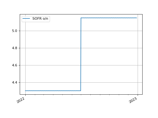
We can plot the overnight rates for the calibrated curve. This curve uses ‘log_linear’ interpolation so the overnight forward rates are constant between node dates.
In [84]: usd_curve.plot("1b", labels=["SOFR o/n"])
Out[84]:
(<Figure size 640x480 with 1 Axes>,
 <Axes: >,
 [<matplotlib.lines.Line2D at 0x170b71a90>])
(Source code, png, hires.png, pdf)
Risk Sensitivities#
Rateslib’s can calculate delta and cross-gamma risks relative to the calibrating Instruments of a Solver. Rateslib also unifies these risks against the FX rates used to create an FXForwards market, to provide a fully consistent risk framework expressed in arbitrary currencies. See the risk framework notes.
Performance wise, because rateslib uses dual number AD upto 2nd order, combined with the appropriate analysis, it is shown to calculate a 150x150 Instrument cross-gamma grid (22,500 elements) from a calculated portfolio NPV in approximately 250ms.
Scheduling#
Necessary functionality is provided natively by rateslib. See:
Utilities#
Rateslib could not function without some utility libraries. These are often referenced in other guides as they arise and can also be linked to from those sections.
Specifically those utilities are:
Cookbook#
This is a collection of more detailed examples and explanations that don’t necessarily fall into any one category. See the Cookbook index.
Advanced Concepts#
These sections describe and exemplify some of the architectural choices in rateslib.
Pricing Mechanisms#
Since rateslib is an object oriented library with object associations we give detailed instructions of the way in which the associations can be constructed in mechanisms.
The key takeway is that when you initialise and create an Instrument you can do one of three things:
Not provide any Curves (or Vol surface) for pricing upfront (
curves=NoInput(0)).Create an explicit association to pre-existing Python objects, e.g.
curves=my_curve.Define some reference to a Curves mapping with strings using
curves="my_curve_id".
If you do 1) then you must provide Curves at price
time: instrument.npv(curves=my_curve).
If you do 2) then you do not need to provide anything further at price time:
instrument.npv(). But you still can provide Curves directly, like for 1), as an override.
If you do 3) then you can provide a Solver which contains the Curves and will
resolve the string mapping: instrument.npv(solver=my_solver). But you can also provide Curves
directly, like for 1), as an override.
Best practice in rateslib is to use 3). This is the safest and most flexible approach and designed to work best with risk sensitivity calculations also.
Mutability#
A proper outline of the mutability of objects is given in mutability.
In summary, best practice is to create new instances and avoid directly overwriting or adding
to class attributes. Don’t mutate a created object unless using an official method to do so,
e.g. FXRates.update or
Curve.update