
Non-Deliverable IRS and XCS: EM Markets#
Rateslib v2.5 introduced non-deliverable IRS and XCS. This page exemplifies how to use these objects to calibrate Curves in those markets. Specifically here we will use ND-IRS and NDXCS to calibrate Indian Rupee Curves.
Key Points
A USD Curve is established in the normal way using US instruments.
An FXForwards market is proposed (uncalibrated) between USD and INR.
The suite of non-deliverable Instruments are constructed and used for calibration.
The Deliverable US Market#
First, we need to establish the baseline US market and the SOFR curve. This is no different to any other tutorial on the matter, so we quickly do this with some of the following SOFR swap data. Just for some variety, this Curve will be interpolated with a log-cubic DF spline.
In [1]: usd = Curve(
   ...:     nodes={
   ...:         dt(2025, 12, 29): 1.0,
   ...:         dt(2026, 12, 29): 1.0,
   ...:         dt(2027, 12, 29): 1.0,
   ...:         dt(2028, 12, 29): 1.0,
   ...:         dt(2029, 12, 29): 1.0,
   ...:         dt(2031, 1, 7): 1.0,
   ...:     },
   ...:     convention="Act360",
   ...:     calendar="nyc",
   ...:     interpolation="spline",
   ...:     id="sofr"
   ...: )
   ...:

In [2]: us_solver = Solver(
   ...:     curves=[usd],
   ...:     instruments=[
   ...:         IRS(dt(2025, 12, 31), "1y", spec="usd_irs", curves="sofr"),
   ...:         IRS(dt(2025, 12, 31), "2y", spec="usd_irs", curves="sofr"),
   ...:         IRS(dt(2025, 12, 31), "3y", spec="usd_irs", curves="sofr"),
   ...:         IRS(dt(2025, 12, 31), "4y", spec="usd_irs", curves="sofr"),
   ...:         IRS(dt(2025, 12, 31), "5y", spec="usd_irs", curves="sofr"),
   ...:     ],
   ...:     s=[3.434, 3.302, 3.314, 3.359, 3.416],
   ...: )
   ...:
SUCCESS: `func_tol` reached after 5 iterations (levenberg_marquardt), `f_val`: 2.988038447678138e-15, `time`: 0.0047s
The Components for the FXForwards#
We are going to use just the 1Y through 5Y instruments, as demonstration, to calibrate the INR market. So our local FBIL Overnight Mumbai Interbank Outright Rate (FBIL-O/N MIBOR) is the following:
In [3]: inr = Curve(
   ...:     nodes={
   ...:         dt(2025, 12, 29): 1.0,
   ...:         dt(2026, 12, 29): 1.0,
   ...:         dt(2027, 12, 29): 1.0,
   ...:         dt(2028, 12, 29): 1.0,
   ...:         dt(2029, 12, 29): 1.0,
   ...:         dt(2031, 1, 7): 1.0,
   ...:     },
   ...:     convention="Act365F",
   ...:     calendar="mum",
   ...:     id="mibor-ois",
   ...: )
   ...:
In order to introduce the necessary degrees of freedom to satisfy the cross-currency market and supply and demand we establish the basis curve:
In [4]: inrusd = Curve(
   ...:     nodes={
   ...:         dt(2025, 12, 29): 1.0,
   ...:         dt(2026, 12, 29): 1.0,
   ...:         dt(2027, 12, 29): 1.0,
   ...:         dt(2028, 12, 29): 1.0,
   ...:         dt(2029, 12, 29): 1.0,
   ...:         dt(2031, 1, 7): 1.0,
   ...:     },
   ...:     convention="Act365F",
   ...:     calendar="all",  # <- no holiday calendar necessary for a cross-currency discount curve.
   ...:     id="inrusd",
   ...: )
   ...:
Finally we put all of the elements together to create the USDINR FXForwards market, note that we have also input the spot USDINR FX rate here as well:
In [5]: fxf = FXForwards(
   ...:     fx_rates=FXRates({"usdinr": 89.9812}, settlement=dt(2025, 12, 31)),
   ...:     fx_curves={"usdusd": usd, "inrinr": inr, "inrusd": inrusd},
   ...: )
   ...:
This object can now be used to forecast any USDINR rate, but it won’t be accurate becuase we haven’t calibrated anything yet! The INR rates are currently all zero on the 2 INR Curves.
In [6]: fxf.rate("usdinr", settlement=dt(2026, 12, 31))
Out[6]: <Dual: 86.953737, (fx_usdinr, sofr0, sofr1, ...), [1.0, 0.4, 89.1, ...]>

In [7]: fxf.swap("usdinr", [dt(2025, 12, 31), dt(2026, 12, 31)])
Out[7]: <Dual: -30274.634161, (fx_usdinr, sofr0, sofr1, ...), [-336.5, 3850.5, 890788.9, ...]>
Calibrating the Curves#
So, we have now reached the point where we can calibrate the INR curves. We have 10 parameters /
degrees of freedom and will therefore require 10 Instruments. We will use 5 NDIRS, which will
calibrate local currency interest rates (the inr Curve) [Bloomberg Moniker IRSWNI1 Curncy],
and 5 NDXCS [Bloomberg Moniker IRUSON1 Curncy] which will effectively calibrate the
cross-currency basis.
Rateslib has added some spec defaults for the purpose of this article, but the keyword
arguments used can be directly observed below:
In [8]: defaults.spec["inr_ndirs"]
Out[8]:
{'frequency': 's',
 'stub': 'shortfront',
 'eom': False,
 'modifier': 'mf',
 'calendar': 'mum',
 'payment_lag': 0,
 'currency': 'usd',
 'convention': 'act365f',
 'leg2_spread_compound_method': 'none_simple',
 'leg2_fixing_method': 'rfr_payment_delay',
 'leg2_method_param': 0,
 'pair': 'usdinr'}

In [9]: defaults.spec["inrusd_ndxcs"]
Out[9]:
{'frequency': 's',
 'stub': 'shortfront',
 'eom': False,
 'modifier': 'mf',
 'calendar': 'mum|fed',
 'payment_lag': 2,
 'currency': 'usd',
 'convention': 'act365f',
 'leg2_convention': 'act360',
 'leg2_spread_compound_method': 'none_simple',
 'leg2_fixing_method': 'rfr_payment_delay',
 'leg2_method_param': 0,
 'fixed': True,
 'pair': 'usdinr'}
To calibrate we must include the previous US Solver, which contains
the mapping to the constructed US SOFR Curve, and we specify the Instruments and the live
market data rates.
In [10]: inr_solver = Solver(
   ....:     pre_solvers=[us_solver],
   ....:     curves=[inr, inrusd],
   ....:     instruments=[
   ....:         IRS(dt(2025, 12, 30), "1Y", spec="inr_ndirs", curves=["mibor-ois", "sofr"]),
   ....:         IRS(dt(2025, 12, 30), "2Y", spec="inr_ndirs", curves=["mibor-ois", "sofr"]),
   ....:         IRS(dt(2025, 12, 30), "3Y", spec="inr_ndirs", curves=["mibor-ois", "sofr"]),
   ....:         IRS(dt(2025, 12, 30), "4Y", spec="inr_ndirs", curves=["mibor-ois", "sofr"]),
   ....:         IRS(dt(2025, 12, 30), "5Y", spec="inr_ndirs", curves=["mibor-ois", "sofr"]),
   ....:         NDXCS(dt(2025, 12, 31), "1Y", spec="inrusd_ndxcs", curves=[None, "sofr", "sofr", "sofr"]),
   ....:         NDXCS(dt(2025, 12, 31), "2Y", spec="inrusd_ndxcs", curves=[None, "sofr", "sofr", "sofr"]),
   ....:         NDXCS(dt(2025, 12, 31), "3Y", spec="inrusd_ndxcs", curves=[None, "sofr", "sofr", "sofr"]),
   ....:         NDXCS(dt(2025, 12, 31), "4Y", spec="inrusd_ndxcs", curves=[None, "sofr", "sofr", "sofr"]),
   ....:         NDXCS(dt(2025, 12, 31), "5Y", spec="inrusd_ndxcs", curves=[None, "sofr", "sofr", "sofr"]),
   ....:     ],
   ....:     s=[
   ....:         5.47, 5.5525, 5.715, 5.835, 5.925, #  <-  IRS rates
   ....:         6.375, 6.335, 6.415, 6.535, 6.595  #  <-  XCS rates
   ....:     ],
   ....:     fx=fxf,
   ....: )
   ....:
SUCCESS: `func_tol` reached after 5 iterations (levenberg_marquardt), `f_val`: 3.2047145174585473e-15, `time`: 0.0260s
What is interesting to note about this particular Solver configuration is that nowhere does the
‘inrusd’ discount Curve enter any Instrument specification. Since these Instruments have
non-deliverable cashflows every discount Curve is the USD SOFR Curve. The key pricing component
here is the fx=fxf object, which is a pricing parameter that is needed and is passed to
all Instruments, and of course it derives forward FX rates using the ‘inrusd’ Curve so
everything is calibrated accurately.
The datasource (DS) for these prices also gives (wide) financial bid/ask for FX swaps and FX forwards.
We can compare these with the FXForwards we have constructed through rateslib (RL)
calibration.
In [11]: df
Out[11]:
  tenor  DS forward  DS swap  RL forward   RL swap
0    1y       92.51    25300       92.58  26021.25
1    2y       95.45    54700       95.44  54540.08
2    3y       98.32    83400       98.48  85015.81
3    4y      101.31   113300      101.84 118578.27
4    5y      104.79   148100      105.06 150773.98
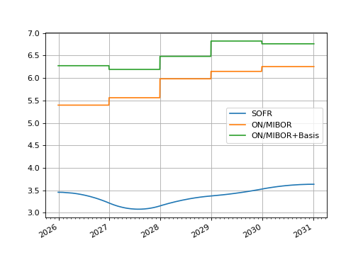
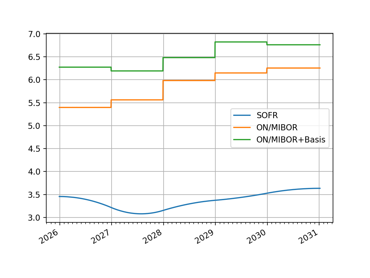
Lets have a look at the calibrate Curves thus far:
In [12]: usd.plot("1b", comparators=[inr, inrusd], labels=["SOFR", "ON/MIBOR", "ON/MIBOR+Basis"])
Out[12]:
(<Figure size 640x480 with 1 Axes>,
 <Axes: >,
 [<matplotlib.lines.Line2D at 0x16d61f230>,
  <matplotlib.lines.Line2D at 0x16d61ecf0>,
  <matplotlib.lines.Line2D at 0x16d61e7b0>])
(Source code, png, hires.png, pdf)
