
Inflation Indexes and Curves 2 (Quantlib comparison)#
This guide replicates and is a comparison to the Quantlib tutorial page at https://www.quantlibguide.com/Inflation%20indexes%20and%20curves.html
Inflation Indexes#
Historical index fixings in rateslib should be indexed to the 1st of the appropriate inflation month.
[1]:
from rateslib import *
from pandas import Series, MultiIndex
[2]:
inflation_fixings = [
    (dt(2022, 1, 1), 110.70),
    (dt(2022, 2, 1), 111.74),
    (dt(2022, 3, 1), 114.46),
    (dt(2022, 4, 1), 115.11),
    (dt(2022, 5, 1), 116.07),
    (dt(2022, 6, 1), 117.01),
    (dt(2022, 7, 1), 117.14),
    (dt(2022, 8, 1), 117.85),
    (dt(2022, 9, 1), 119.26),
    (dt(2022, 10, 1), 121.03),
    (dt(2022, 11, 1), 120.95),
    (dt(2022, 12, 1), 120.52),
    (dt(2023, 1, 1), 120.27),
    (dt(2023, 2, 1), 121.24),
    (dt(2023, 3, 1), 122.34),
    (dt(2023, 4, 1), 123.12),
    (dt(2023, 5, 1), 123.15),
    (dt(2023, 6, 1), 123.47),
    (dt(2023, 7, 1), 123.36),
    (dt(2023, 8, 1), 124.03),
    (dt(2023, 9, 1), 124.43),
    (dt(2023, 10, 1), 124.54),
    (dt(2023, 11, 1), 123.85),
    (dt(2023, 12, 1), 124.05),
    (dt(2024, 1, 1), 123.60),
    (dt(2024, 2, 1), 124.37),
    (dt(2024, 3, 1), 125.31),
    (dt(2024, 4, 1), 126.05),
]
dates, values = zip(*inflation_fixings)
fixings.add("cpi_fixings", Series(values, dates))
Rateslib contains an index_value method that will determine such for a given reference value date and other common parameters.
[3]:
index_value(
    index_lag=0,
    index_method="monthly",
    index_fixings="cpi_fixings",
    index_date=dt(2024, 3, 15)
)
[3]:
np.float64(125.31)
For example to replicate the Quantlib example of a lagged reference date we can use:
[4]:
index_value(
    index_lag=3,
    index_method="daily",
    index_fixings="cpi_fixings",
    index_date=dt(2024, 5, 15)
)
[4]:
np.float64(124.79451612903226)
Inflation Curves#
Create a nominal discount curve for cashflows. Calibrated to a 3% continuously compounded rate.
[5]:
nominal_curve = Curve(
    nodes={dt(2024, 5, 11): 1.0, dt(2074, 5, 18): 1.0},
    interpolation="log_linear",
    convention="Act365F",
    id="discount"
)
solver1 = Solver(
    curves=[nominal_curve],
    instruments=[Value(dt(2074, 5, 11), metric="cc_zero_rate", curves="discount")],
    s=[3.0],
    id="rates",
    instrument_labels=["nominal"],
)
SUCCESS: `func_tol` reached after 7 iterations (levenberg_marquardt), `f_val`: 7.1651768419373015e-12, `time`: 0.0011s
Now create an inflation curve, based on the last known CPI print, calibrated with zero coupon inflation swaps rates. Notice that an inflation curve starts as of the last known fixing as its index_base. This is similar to Quantlib, not be design, but by necessity since this is the only information we have that can define the start of the curve.
[6]:
inflation_curve = Curve(
    nodes={
        dt(2024, 4, 1): 1.0,  # <- last known inflation print.
        dt(2025, 5, 11): 1.0,  # 1y
        dt(2026, 5, 11): 1.0,  # 2y
        dt(2027, 5, 11): 1.0,  # 3y
        dt(2028, 5, 11): 1.0,  # 4y
        dt(2029, 5, 11): 1.0,  # 5y
        dt(2031, 5, 11): 1.0,  # 7y
        dt(2034, 5, 11): 1.0,  # 10y
        dt(2036, 5, 11): 1.0,  # 12y
        dt(2039, 5, 11): 1.0,  # 15y
        dt(2044, 5, 11): 1.0,  # 20y
        dt(2049, 5, 11): 1.0,  # 25y
        dt(2054, 5, 11): 1.0,  # 30y
        dt(2064, 5, 11): 1.0,  # 40y
        dt(2074, 5, 11): 1.0,  # 50y
    },
    interpolation="log_linear",
    convention="Act365F",
    index_base=126.05,
    index_lag=0,
    id="inflation"
)
solver = Solver(
    pre_solvers=[solver1],
    curves=[inflation_curve],
    instruments=[
        ZCIS(dt(2024, 5, 11), "1y", spec="eur_zcis", curves=["inflation", "discount"], leg2_index_fixings="cpi_fixings"),
        ZCIS(dt(2024, 5, 11), "2y", spec="eur_zcis", curves=["inflation", "discount"], leg2_index_fixings="cpi_fixings"),
        ZCIS(dt(2024, 5, 11), "3y", spec="eur_zcis", curves=["inflation", "discount"], leg2_index_fixings="cpi_fixings"),
        ZCIS(dt(2024, 5, 11), "4y", spec="eur_zcis", curves=["inflation", "discount"], leg2_index_fixings="cpi_fixings"),
        ZCIS(dt(2024, 5, 11), "5y", spec="eur_zcis", curves=["inflation", "discount"], leg2_index_fixings="cpi_fixings"),
        ZCIS(dt(2024, 5, 11), "7y", spec="eur_zcis", curves=["inflation", "discount"], leg2_index_fixings="cpi_fixings"),
        ZCIS(dt(2024, 5, 11), "10y", spec="eur_zcis", curves=["inflation", "discount"], leg2_index_fixings="cpi_fixings"),
        ZCIS(dt(2024, 5, 11), "12y", spec="eur_zcis", curves=["inflation", "discount"], leg2_index_fixings="cpi_fixings"),
        ZCIS(dt(2024, 5, 11), "15y", spec="eur_zcis", curves=["inflation", "discount"], leg2_index_fixings="cpi_fixings"),
        ZCIS(dt(2024, 5, 11), "20y", spec="eur_zcis", curves=["inflation", "discount"], leg2_index_fixings="cpi_fixings"),
        ZCIS(dt(2024, 5, 11), "25y", spec="eur_zcis", curves=["inflation", "discount"], leg2_index_fixings="cpi_fixings"),
        ZCIS(dt(2024, 5, 11), "30y", spec="eur_zcis", curves=["inflation", "discount"], leg2_index_fixings="cpi_fixings"),
        ZCIS(dt(2024, 5, 11), "40y", spec="eur_zcis", curves=["inflation", "discount"], leg2_index_fixings="cpi_fixings"),
        ZCIS(dt(2024, 5, 11), "50y", spec="eur_zcis", curves=["inflation", "discount"], leg2_index_fixings="cpi_fixings"),
    ],
    s=[2.93, 2.95, 2.965, 2.98, 3.0, 3.06, 3.175, 3.243, 3.293, 3.338, 3.348, 3.348, 3.308, 3.228],
    instrument_labels=["1y", "2y", "3y", "4y", "5y", "7y", "10y", "12y", "15", "20y", "25y", "30y", "40y", "50y"],
    id="zcis",
)
SUCCESS: `func_tol` reached after 8 iterations (levenberg_marquardt), `f_val`: 1.4302416694642844e-17, `time`: 0.0153s
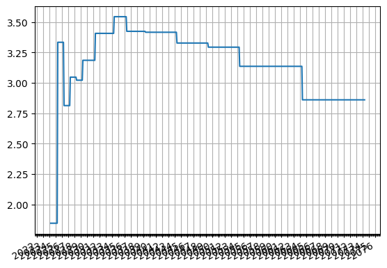
The data can be output to a table or plotted as below.
[7]:
inflation_curve.plot("1m")
[7]:
(<Figure size 640x480 with 1 Axes>,
 <Axes: >,
 [<matplotlib.lines.Line2D at 0x116a416a0>])
[8]:
inflation_curve.plot_index(right=dt(2030, 6, 1))
[8]:
(<Figure size 640x480 with 1 Axes>,
 <Axes: >,
 [<matplotlib.lines.Line2D at 0x1176e7620>])
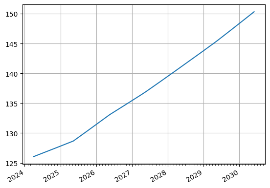
Some of the forecast values from the curve can be obtained directly from Curve methods.
[9]:
inflation_curve.index_value(dt(2027, 4, 1), index_lag=3, index_method="monthly")
[9]:
<Dual: 135.440324, (inflation0, inflation1, inflation2, ...), [-0.0, -0.0, -50.9, ...]>
[10]:
inflation_curve.index_value(dt(2027, 4, 1), index_lag=0, index_method="monthly")
[10]:
<Dual: 136.382058, (inflation0, inflation1, inflation2, ...), [-0.0, -0.0, -15.8, ...]>
[11]:
inflation_curve.index_value(dt(2027, 5, 15), index_lag=3, index_method="daily")
[11]:
<Dual: 135.896278, (inflation0, inflation1, inflation2, ...), [0.0, 0.0, -33.9, ...]>
Seasonality#
The way rateslib handles seasonality is to replicate it via its CompositeCurve framework. With this approach, adding seasonality can be done in a multitude of ways, but since Quantlib has used seasonaility factors we will synthesize that approach within rateslib’s framework. We create a new curve with node dates reflecting the key dates used by Quantlib.
The theory here for rateslib is as follows.
A discount factor on a rateslib CompositeCurve is very approximately the product of the discount factors of its contained curves (c1 and c2):
The CompositeCurve index value takes its index base from the first (main) curve in its composition, therefore the index value is calculated according to:
If we set the index base on the seasonality curve (c2) exactly to 1.0 this equation reduces to:
So the index value on the CompositeCurve equals the product of the two index values.
Thus, if we set the set the index values on the seasonality curve (c2) directly they can act directly as multipliers to the underlying inflation values on the inflation curve. This seasonality curve can be calibrated using a Solver, and in this particular case (to match Quantlib) they are calibrated directly with index values.
Here we add the same seasonality factors in years 2025, 2026 and 2027.
[12]:
season = Curve(
    nodes={
        dt(2024, 4, 1): 1.0,
        dt(2024, 12, 1): 1.0,
        **{dt(2025, _, 1): 1.0 for _ in range(1, 13)},
        **{dt(2026, _, 1): 1.0 for _ in range(1, 13)},
        **{dt(2027, _, 1): 1.0 for _ in range(1, 13)},
        dt(2074, 5, 11): 1.0,
    },
    interpolation="log_linear",
    convention="Act365F",
    index_base=1.0,  #  <- as per theory above
    index_lag=0,  # <- matches the main inflation curve
    id="seasonality"
)
The seasonality factors will be added by directly inserting index values at specific dates.
[13]:
yearly_multipliers = [
    1.003245,
    1.001994,
    0.999715,
    1.000495,
    1.000929,
    0.998687,
    0.995949,
    0.994682,
    0.995949,
    1.000519,
    1.003705,
    1.004186,
]
season_solver = Solver(
    curves=[season],
    instruments=\
        [Value(dt(2024, 12, 1), curves=[season], metric="index_value")] +\
        [Value(dt(2025, _, 1), curves=[season], metric="index_value") for _ in range(1, 13)] +\
        [Value(dt(2026, _, 1), curves=[season], metric="index_value") for _ in range(1, 13)] +\
        [Value(dt(2027, _, 1), curves=[season], metric="index_value") for _ in range(1, 13)],
    s=[1.0] + yearly_multipliers*3
)
SUCCESS: `func_tol` reached after 8 iterations (levenberg_marquardt), `f_val`: 1.290941550558499e-12, `time`: 0.0206s
[14]:
season.plot("1b", left=dt(2024, 4, 1), right=dt(2028, 4, 1))
[14]:
(<Figure size 640x480 with 1 Axes>,
 <Axes: >,
 [<matplotlib.lines.Line2D at 0x11785e510>])
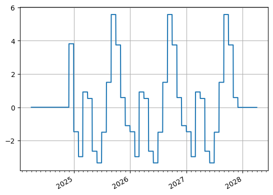
Once the seasonality is designed it must be composited with an underlying inflation curve and the instruments re-solved
[15]:
inflation_with_season = CompositeCurve([inflation_curve, season], id="inflation_s")
[16]:
solver = Solver(
    pre_solvers=[solver1],  # nominal discount curve
    curves=[inflation_with_season, inflation_curve],
    instruments=[
        ZCIS(dt(2024, 5, 11), "1y", spec="eur_zcis", curves=["inflation_s", "discount"], leg2_index_fixings="cpi_fixings"),
        ZCIS(dt(2024, 5, 11), "2y", spec="eur_zcis", curves=["inflation_s", "discount"], leg2_index_fixings="cpi_fixings"),
        ZCIS(dt(2024, 5, 11), "3y", spec="eur_zcis", curves=["inflation_s", "discount"], leg2_index_fixings="cpi_fixings"),
        ZCIS(dt(2024, 5, 11), "4y", spec="eur_zcis", curves=["inflation_s", "discount"], leg2_index_fixings="cpi_fixings"),
        ZCIS(dt(2024, 5, 11), "5y", spec="eur_zcis", curves=["inflation_s", "discount"], leg2_index_fixings="cpi_fixings"),
        ZCIS(dt(2024, 5, 11), "7y", spec="eur_zcis", curves=["inflation_s", "discount"], leg2_index_fixings="cpi_fixings"),
        ZCIS(dt(2024, 5, 11), "10y", spec="eur_zcis", curves=["inflation_s", "discount"], leg2_index_fixings="cpi_fixings"),
        ZCIS(dt(2024, 5, 11), "12y", spec="eur_zcis", curves=["inflation_s", "discount"], leg2_index_fixings="cpi_fixings"),
        ZCIS(dt(2024, 5, 11), "15y", spec="eur_zcis", curves=["inflation_s", "discount"], leg2_index_fixings="cpi_fixings"),
        ZCIS(dt(2024, 5, 11), "20y", spec="eur_zcis", curves=["inflation_s", "discount"], leg2_index_fixings="cpi_fixings"),
        ZCIS(dt(2024, 5, 11), "25y", spec="eur_zcis", curves=["inflation_s", "discount"], leg2_index_fixings="cpi_fixings"),
        ZCIS(dt(2024, 5, 11), "30y", spec="eur_zcis", curves=["inflation_s", "discount"], leg2_index_fixings="cpi_fixings"),
        ZCIS(dt(2024, 5, 11), "40y", spec="eur_zcis", curves=["inflation_s", "discount"], leg2_index_fixings="cpi_fixings"),
        ZCIS(dt(2024, 5, 11), "50y", spec="eur_zcis", curves=["inflation_s", "discount"], leg2_index_fixings="cpi_fixings"),
    ],
    s=[2.93, 2.95, 2.965, 2.98, 3.0, 3.06, 3.175, 3.243, 3.293, 3.338, 3.348, 3.348, 3.308, 3.228],
    instrument_labels=["1y", "2y", "3y", "4y", "5y", "7y", "10y", "12y", "15y", "20y", "25y", "30y", "40y", "50y"],
    id="zcis",
)
SUCCESS: `func_tol` reached after 5 iterations (levenberg_marquardt), `f_val`: 1.7223655493350175e-13, `time`: 0.0145s
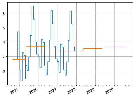
[17]:
inflation_with_season.plot("1b", comparators=[inflation_curve], left=dt(2024, 9, 1), right=dt(2030, 9, 1))
[17]:
(<Figure size 640x480 with 1 Axes>,
 <Axes: >,
 [<matplotlib.lines.Line2D at 0x117b1eba0>,
  <matplotlib.lines.Line2D at 0x117b1ecf0>])
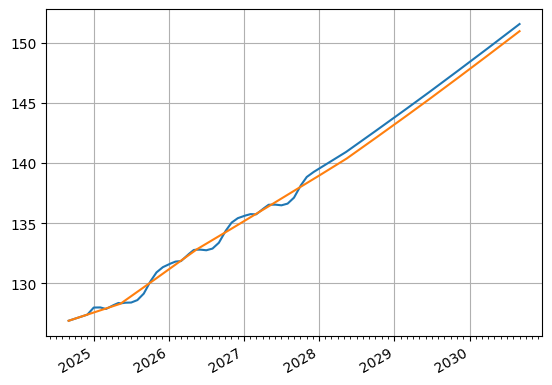
[18]:
inflation_with_season.plot_index(comparators=[inflation_curve], left=dt(2024, 9, 1), right=dt(2030, 9, 1))
[18]:
(<Figure size 640x480 with 1 Axes>,
 <Axes: >,
 [<matplotlib.lines.Line2D at 0x120994ec0>,
  <matplotlib.lines.Line2D at 0x120995010>])
New sampled values#
[19]:
inflation_with_season.index_value(dt(2027, 4, 1), index_lag=3, index_method="monthly")
[19]:
<Dual: 135.613192, (inflation0, inflation1, inflation2, ...), [0.0, 0.0, -50.9, ...]>
[20]:
inflation_with_season.index_value(dt(2027, 4, 1), index_lag=0, index_method="monthly")
[20]:
<Dual: 136.170810, (inflation0, inflation1, inflation2, ...), [0.0, 0.0, -15.7, ...]>
[21]:
inflation_with_season.index_value(dt(2027, 5, 15), index_lag=3, index_method="daily")
[21]:
<Dual: 135.754993, (inflation0, inflation1, inflation2, ...), [0.0, 0.0, -33.8, ...]>
The trick here is obviously to find a representation of a seasonality curve that matches one’s expectation of seasonality adjustments. Here, a Solver calibration was used to separately solve the seasonality curve to inflation rate adjustments.
[22]:
for i, date in enumerate([dt(2025, _, 1) for _ in range(1, 13)]+[dt(2026, _, 1) for _ in range(1, 13)]):
    a = inflation_curve.index_value(date, index_lag=0, index_method="monthly")
    b = inflation_with_season.index_value(date, index_lag=0, index_method="monthly")
    print(f"Date: {date}, Inflation curve: {float(a):.5f}, With seasonality: {float(b):.5f}, Multiplier: {float(b/a):.7f}, Intended Multiplier: {yearly_multipliers[i%12]:.7f}")
Date: 2025-01-01 00:00:00, Inflation curve: 127.58510, With seasonality: 127.99907, Multiplier: 1.0032447, Intended Multiplier: 1.0032450
Date: 2025-02-01 00:00:00, Inflation curve: 127.75932, With seasonality: 128.01404, Multiplier: 1.0019938, Intended Multiplier: 1.0019940
Date: 2025-03-01 00:00:00, Inflation curve: 127.91688, With seasonality: 127.88042, Multiplier: 0.9997150, Intended Multiplier: 0.9997150
Date: 2025-04-01 00:00:00, Inflation curve: 128.09155, With seasonality: 128.15494, Multiplier: 1.0004949, Intended Multiplier: 1.0004950
Date: 2025-05-01 00:00:00, Inflation curve: 128.26081, With seasonality: 128.37995, Multiplier: 1.0009289, Intended Multiplier: 1.0009290
Date: 2025-06-01 00:00:00, Inflation curve: 128.56987, With seasonality: 128.40108, Multiplier: 0.9986871, Intended Multiplier: 0.9986870
Date: 2025-07-01 00:00:00, Inflation curve: 128.93158, With seasonality: 128.40934, Multiplier: 0.9959495, Intended Multiplier: 0.9959490
Date: 2025-08-01 00:00:00, Inflation curve: 129.30641, With seasonality: 128.61884, Multiplier: 0.9946826, Intended Multiplier: 0.9946820
Date: 2025-09-01 00:00:00, Inflation curve: 129.68234, With seasonality: 129.15706, Multiplier: 0.9959495, Intended Multiplier: 0.9959490
Date: 2025-10-01 00:00:00, Inflation curve: 130.04718, With seasonality: 130.11466, Multiplier: 1.0005189, Intended Multiplier: 1.0005190
Date: 2025-11-01 00:00:00, Inflation curve: 130.42525, With seasonality: 130.90842, Multiplier: 1.0037046, Intended Multiplier: 1.0037050
Date: 2025-12-01 00:00:00, Inflation curve: 130.79218, With seasonality: 131.33961, Multiplier: 1.0041855, Intended Multiplier: 1.0041860
Date: 2026-01-01 00:00:00, Inflation curve: 131.17243, With seasonality: 131.59803, Multiplier: 1.0032446, Intended Multiplier: 1.0032450
Date: 2026-02-01 00:00:00, Inflation curve: 131.55378, With seasonality: 131.81606, Multiplier: 1.0019938, Intended Multiplier: 1.0019940
Date: 2026-03-01 00:00:00, Inflation curve: 131.89917, With seasonality: 131.86159, Multiplier: 0.9997150, Intended Multiplier: 0.9997150
Date: 2026-04-01 00:00:00, Inflation curve: 132.28264, With seasonality: 132.34811, Multiplier: 1.0004949, Intended Multiplier: 1.0004950
Date: 2026-05-01 00:00:00, Inflation curve: 132.65479, With seasonality: 132.77801, Multiplier: 1.0009289, Intended Multiplier: 1.0009290
Date: 2026-06-01 00:00:00, Inflation curve: 132.99141, With seasonality: 132.81681, Multiplier: 0.9986872, Intended Multiplier: 0.9986870
Date: 2026-07-01 00:00:00, Inflation curve: 133.29532, With seasonality: 132.75542, Multiplier: 0.9959495, Intended Multiplier: 0.9959490
Date: 2026-08-01 00:00:00, Inflation curve: 133.61010, With seasonality: 132.89966, Multiplier: 0.9946827, Intended Multiplier: 0.9946820
Date: 2026-09-01 00:00:00, Inflation curve: 133.92562, With seasonality: 133.38316, Multiplier: 0.9959495, Intended Multiplier: 0.9959490
Date: 2026-10-01 00:00:00, Inflation curve: 134.23168, With seasonality: 134.30133, Multiplier: 1.0005189, Intended Multiplier: 1.0005190
Date: 2026-11-01 00:00:00, Inflation curve: 134.54867, With seasonality: 135.04711, Multiplier: 1.0037045, Intended Multiplier: 1.0037050
Date: 2026-12-01 00:00:00, Inflation curve: 134.85614, With seasonality: 135.42058, Multiplier: 1.0041855, Intended Multiplier: 1.0041860
Inflation Swap and DV01#
We can easily construct a ZCIS or other type of inflation based instrument and use the native delta and gamma methods associated with a Solver to extract risk sensitivities.
[23]:
zcis = ZCIS(dt(2024, 3, 11), "4y", spec="eur_zcis", curves=["inflation_s", "discount"], fixed_rate=3.0, leg2_index_fixings="cpi_fixings")
[24]:
zcis.rate(solver=solver)
[24]:
<Dual: 2.926124, (inflation0, inflation1, inflation2, ...), [0.0, 0.0, 0.0, ...]>
[25]:
zcis.npv(solver=solver)
[25]:
<Dual: -2874.505227, (inflation0, inflation1, inflation2, ...), [0.0, 0.0, 0.0, ...]>
[26]:
df = zcis.delta(solver=solver)
descriptors = df.agg(["sum"])
descriptors.index = MultiIndex.from_tuples([("sum", "sum", "sum")])
df.style.format(precision=0).concat(descriptors.style.format(precision=0))
[26]:
| local_ccy | eur | ||
|---|---|---|---|
| display_ccy | eur | ||
| type | solver | label | |
| instruments | rates | nominal | 1 |
| zcis | 1y | 4 | |
| 2y | -23 | ||
| 3y | 93 | ||
| 4y | 298 | ||
| 5y | -0 | ||
| 7y | -0 | ||
| 10y | 0 | ||
| 12y | 0 | ||
| 15y | 0 | ||
| 20y | 0 | ||
| 25y | -0 | ||
| 30y | 0 | ||
| 40y | -0 | ||
| 50y | -0 | ||
| sum | sum | sum | 373 |
This risk display shows no exposure to the seasonality configuration becuase the Solver that was used to calibrate the seasonality was not added as a pre_solver to the Solver used in the last step. Therefore it treats the seasonality as a constant and not as variable to which risk sensitivities can be obtained.
To observe the change, simply replace pre_solvers=[solver1] with pre_solvers=[solver1, season_solver], in the above Solver and re run the cells.
[27]:
zcis.gamma(solver=solver).style.format(precision=1)
[27]:
| type | instruments | ||||||||||||||||||
|---|---|---|---|---|---|---|---|---|---|---|---|---|---|---|---|---|---|---|---|
| solver | rates | zcis | |||||||||||||||||
| label | nominal | 1y | 2y | 3y | 4y | 5y | 7y | 10y | 12y | 15y | 20y | 25y | 30y | 40y | 50y | ||||
| local_ccy | display_ccy | type | solver | label | |||||||||||||||
| eur | eur | instruments | rates | nominal | -0.0 | -0.0 | 0.0 | -0.0 | -0.1 | 0.0 | 0.0 | -0.0 | -0.0 | -0.0 | -0.0 | -0.0 | -0.0 | 0.0 | 0.0 |
| zcis | 1y | -0.0 | -0.0 | -0.0 | 0.0 | 0.0 | -0.0 | -0.0 | 0.0 | 0.0 | 0.0 | 0.0 | 0.0 | 0.0 | -0.0 | -0.0 | |||
| 2y | 0.0 | -0.0 | 0.0 | -0.0 | -0.0 | 0.0 | 0.0 | -0.0 | -0.0 | -0.0 | -0.0 | -0.0 | -0.0 | 0.0 | 0.0 | ||||
| 3y | -0.0 | 0.0 | -0.0 | -0.0 | 0.0 | -0.0 | -0.0 | -0.0 | 0.0 | 0.0 | 0.0 | 0.0 | 0.0 | -0.0 | -0.0 | ||||
| 4y | -0.1 | 0.0 | -0.0 | 0.0 | 0.1 | -0.0 | -0.0 | 0.0 | 0.0 | 0.0 | 0.0 | 0.0 | 0.0 | -0.0 | -0.0 | ||||
| 5y | 0.0 | -0.0 | 0.0 | -0.0 | -0.0 | 0.0 | -0.0 | -0.0 | 0.0 | -0.0 | 0.0 | -0.0 | 0.0 | 0.0 | -0.0 | ||||
| 7y | 0.0 | -0.0 | 0.0 | -0.0 | -0.0 | -0.0 | 0.0 | 0.0 | -0.0 | 0.0 | -0.0 | 0.0 | -0.0 | -0.0 | 0.0 | ||||
| 10y | -0.0 | 0.0 | -0.0 | -0.0 | 0.0 | -0.0 | 0.0 | -0.0 | 0.0 | -0.0 | 0.0 | -0.0 | 0.0 | 0.0 | -0.0 | ||||
| 12y | -0.0 | 0.0 | -0.0 | 0.0 | 0.0 | 0.0 | -0.0 | 0.0 | -0.0 | 0.0 | -0.0 | 0.0 | -0.0 | -0.0 | 0.0 | ||||
| 15y | -0.0 | 0.0 | -0.0 | 0.0 | 0.0 | -0.0 | 0.0 | -0.0 | 0.0 | -0.0 | 0.0 | -0.0 | 0.0 | 0.0 | -0.0 | ||||
| 20y | -0.0 | 0.0 | -0.0 | 0.0 | 0.0 | 0.0 | -0.0 | 0.0 | -0.0 | 0.0 | -0.0 | 0.0 | -0.0 | -0.0 | 0.0 | ||||
| 25y | -0.0 | 0.0 | -0.0 | 0.0 | 0.0 | -0.0 | 0.0 | -0.0 | 0.0 | -0.0 | 0.0 | -0.0 | 0.0 | 0.0 | -0.0 | ||||
| 30y | -0.0 | 0.0 | -0.0 | 0.0 | 0.0 | 0.0 | -0.0 | 0.0 | -0.0 | 0.0 | -0.0 | 0.0 | -0.0 | -0.0 | 0.0 | ||||
| 40y | 0.0 | -0.0 | 0.0 | -0.0 | -0.0 | 0.0 | -0.0 | 0.0 | -0.0 | 0.0 | -0.0 | 0.0 | -0.0 | 0.0 | -0.0 | ||||
| 50y | 0.0 | -0.0 | 0.0 | -0.0 | -0.0 | -0.0 | 0.0 | -0.0 | 0.0 | -0.0 | 0.0 | -0.0 | 0.0 | -0.0 | 0.0 | ||||
[ ]: