
User Guide#
Where to start?#
It is important to understand that this library tends to follow the typical framework:
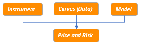
This means that financial instrument specification, curve and/or surface construction from market data including foreign exchange (FX) will permit pricing metrics and risk sensitivity. These functionalities are interlinked and potentially dependent upon each other. This guide’s intention is to introduce them in a structured way and give typical examples how they are used in practice.
Note
If you see this icon  at any point after a section it will link to a section in the
rateslib-excel documentation which may demonstrate the equivalent Python example in Excel.
at any point after a section it will link to a section in the
rateslib-excel documentation which may demonstrate the equivalent Python example in Excel.
Let’s start with the fundamental constructors Curve and Instrument.
A trivial example#
For example, we can construct Curves in many different ways: here we create one by directly specifying discount factors (DFs) on certain node dates (sometimes called pillar dates in other publications).
In [1]: from rateslib import *

In [2]: usd_curve = Curve(
   ...:     nodes={
   ...:         dt(2022, 1, 1): 1.0,
   ...:         dt(2022, 7, 1): 0.98,
   ...:         dt(2023, 1, 1): 0.95
   ...:     },
   ...:     calendar="nyc",
   ...:     id="sofr",
   ...: )
   ...:
We can then construct an Instrument. Here we create a short dated
RFR interest rate swap (IRS) using the conventional market specification
rateslib offers many examples of Instrument specifications as all seen
here in defaults.
In [3]: irs = IRS(
   ...:     effective=dt(2022, 2, 15),
   ...:     termination="6m",
   ...:     notional=1000000000,
   ...:     fixed_rate=2.0,
   ...:     spec="usd_irs"
   ...: )
   ...:
We can value the IRS with the Curve in its local currency (USD) by default, and see the generated cashflows.
In [4]: irs.npv(usd_curve)
Out[4]: 12629097.829705866
In [5]: irs.cashflows(usd_curve)
Out[5]:
               Type Period  Ccy  Acc Start    Acc End    Payment Convention  DCF       Notional   DF Collateral  Rate  Spread     Cashflow         NPV  FX Rate     NPV Ccy
leg1 0  FixedPeriod   Stub  USD 2022-02-15 2022-08-15 2022-08-17     act360 0.50  1000000000.00 0.97       None  2.00     NaN -10055555.56 -9776494.15     1.00 -9776494.15
leg2 0  FloatPeriod   Stub  USD 2022-02-15 2022-08-15 2022-08-17     act360 0.50 -1000000000.00 0.97       None  4.58    0.00  23045139.84 22405591.98     1.00 22405591.98
Quick look at FX#
Spot rates and conversion#
The above values were all calculated and displayed in USD. That is the default
currency in rateslib and the local currency of the swap. We can convert this value to another
currency using the FXRates class. This is a basic class which is
parametrised by some exchange rates.
In [6]: fxr = FXRates({"eurusd": 1.05, "gbpusd": 1.25})

In [7]: fxr.rates_table()
Out[7]:
     usd  eur  gbp
usd 1.00 0.95 0.80
eur 1.05 1.00 0.84
gbp 1.25 1.19 1.00
We now have a mechanism by which to specify values in other currencies.
In [8]: irs.npv(usd_curve, fx=fxr, base="usd")
Out[8]: 12629097.829705866

In [9]: irs.npv(usd_curve, fx=fxr, base="eur")
Out[9]: <Dual: 12027712.218767, (fx_eurusd), [-11454964.0]>
One observes that the value returned here is not a float but a Dual
which is part of rateslib’s AD framework. This is the first example of capturing a
sensitivity, which here denotes the sensitivity of the EUR NPV relative to the EURUSD FX rate.
One can read more about this particular treatment of FX
here and more generally about the dual AD framework here.
FX forwards#
For multi-currency derivatives we need more than basic, spot exchange rates.
We can also create an
FXForwards class. This stores the FX rates and the interest
rates curves that are used for all the FX-interest rate parity derivations. With these
we can calculate forward FX rates and also ad-hoc FX swap rates.
When defining the fx_curves dict mapping, the key “eurusd” should be interpreted as; the
Curve for EUR cashflows, collateralised in USD, and similarly for other entries.
In [10]: eur_curve = Curve({
   ....:     dt(2022, 1, 1): 1.0,
   ....:     dt(2022, 7, 1): 0.972,
   ....:     dt(2023, 1, 1): 0.98},
   ....:     calendar="tgt",
   ....: )
   ....:

In [11]: eurusd_curve = Curve({
   ....:     dt(2022, 1, 1): 1.0,
   ....:     dt(2022, 7, 1): 0.973,
   ....:     dt(2023, 1, 1): 0.981}
   ....: )
   ....:

In [12]: fxf = FXForwards(
   ....:     fx_rates=FXRates({"eurusd": 1.05}, settlement=dt(2022, 1, 1)),
   ....:     fx_curves={
   ....:         "usdusd": usd_curve,
   ....:         "eureur": eur_curve,
   ....:         "eurusd": eurusd_curve,
   ....:     }
   ....: )
   ....:

In [13]: fxf.rate("eurusd", settlement=dt(2023, 1, 1))
Out[13]: <Dual: 1.084263, (fx_eurusd), [1.0]>

In [14]: fxf.swap("eurusd", settlements=[dt(2022, 2, 1), dt(2022, 5, 1)])
Out[14]: <Dual: -36.900308, (fx_eurusd), [-35.1]>
FXForwards objects are comprehensive and more information regarding all of the FX features is available in this link.
More about instruments#
We saw an example of the IRS instrument above.
A complete guide for all of the Instruments is available in
this link. It is
recommended to also, in advance, review Periods and
then Legs, since
the documentation for these building blocks provides technical descriptions of the
parameters that are used to build up the instruments.
Multi-currency instruments#
Let’s take a look at an example of a multi-currency instrument: the
FXSwap. All instruments have a mid-market pricing
function rate(). Keeping a
consistent function name across all Instruments allows any of them to be used within a
Solver to calibrate Curves around target mid-market rates.
This FXSwap Instrument construction prices to the same mid-market rate as the ad-hox swap rate used in the example above (as expected).
In [15]: fxs = FXSwap(
   ....:     effective=dt(2022, 2, 1),
   ....:     termination="3m",  # May-1 is a holiday, May-2 is business end date.
   ....:     pair="eurusd",
   ....:     notional=20e6,
   ....:     calendar="tgt|fed",
   ....: )
   ....:

In [16]: fxs.rate(curves=[None, eurusd_curve, None, usd_curve], fx=fxf)
Out[16]: <Dual: -37.314180, (fx_eurusd), [-35.5]>
Securities and bonds#
A very common instrument in financial investing is a FixedRateBond.
At time of writing the on-the-run 10Y US treasury was the 3.875% Aug 2033 bond. Here we can
construct this using the street convention and derive the price from yield-to-maturity and
risk calculations.
In [17]: fxb = FixedRateBond(
   ....:     effective=dt(2023, 8, 15),
   ....:     termination=dt(2033, 8, 15),
   ....:     fixed_rate=3.875,
   ....:     spec="ust"
   ....: )
   ....:

In [18]: fxb.accrued(settlement=dt(2025, 2, 14))
Out[18]: 1.9269701086956519

In [19]: fxb.price(ytm=4.0, settlement=dt(2025, 2, 14))
Out[19]: 99.10641380057267

In [20]: fxb.duration(ytm=4.0, settlement=dt(2025, 2, 14), metric="duration")
Out[20]: 7.178560455252011

In [21]: fxb.duration(ytm=4.0, settlement=dt(2025, 2, 14), metric="modified")
Out[21]: 7.037804367894129

In [22]: fxb.duration(ytm=4.0, settlement=dt(2025, 2, 14), metric="risk")
Out[22]: 7.11053190579773
There are some interesting Cookbook articles
on BondFuture and cheapest-to-deliver (CTD) analysis.
Calibrating curves with a solver#
The guide for Constructing Curves introduces the main
curve classes,
Curve, LineCurve, and
IndexCurve. It also touches on some of the more
advanced curves CompositeCurve,
ProxyCurve, and MultiCsaCurve.
Calibrating curves is a very natural thing to do in fixed income. We typically use market prices of commonly traded instruments to set values. FX Volatility Smiles and FX Volatility Surfaces are also calibrated using the exact same optimising algorithms.
Below we demonstrate how to calibrate the Curve that
we created above in the initial trivial example using SOFR swap market data. First, we
are reminded of the discount factors (DFs) which were manually set on that curve.
In [23]: usd_curve.nodes
Out[23]:
{datetime.datetime(2022, 1, 1, 0, 0): 1.0,
 datetime.datetime(2022, 7, 1, 0, 0): 0.98,
 datetime.datetime(2023, 1, 1, 0, 0): 0.95}
Now we will instruct a Solver to recalibrate those value to match
a set of prices, s. The calibrating Instruments associated with those prices are 6M and 1Y IRSs.
In [24]: usd_args = dict(
   ....:     effective=dt(2022, 1, 1),
   ....:     spec="usd_irs",
   ....:     curves="sofr"
   ....: )
   ....:

In [25]: solver = Solver(
   ....:     curves=[usd_curve],
   ....:     instruments=[
   ....:         IRS(**usd_args, termination="6M"),
   ....:         IRS(**usd_args, termination="1Y"),
   ....:     ],
   ....:     s=[4.35, 4.85],
   ....:     instrument_labels=["6M", "1Y"],
   ....:     id="us_rates"
   ....: )
   ....:
SUCCESS: `func_tol` reached after 3 iterations (levenberg_marquardt), `f_val`: 3.0486413284865872e-15, `time`: 0.0021s
Solving was a success! Observe that the DFs on the Curve have been updated:
In [26]: usd_curve.nodes
Out[26]:
{datetime.datetime(2022, 1, 1, 0, 0): <Dual: 1.000000, (sofr0, sofr1, sofr2), [1.0, 0.0, 0.0]>,
 datetime.datetime(2022, 7, 1, 0, 0): <Dual: 0.978595, (sofr0, sofr1, sofr2), [0.0, 1.0, 0.0]>,
 datetime.datetime(2023, 1, 1, 0, 0): <Dual: 0.953176, (sofr0, sofr1, sofr2), [0.0, 0.0, 1.0]>}
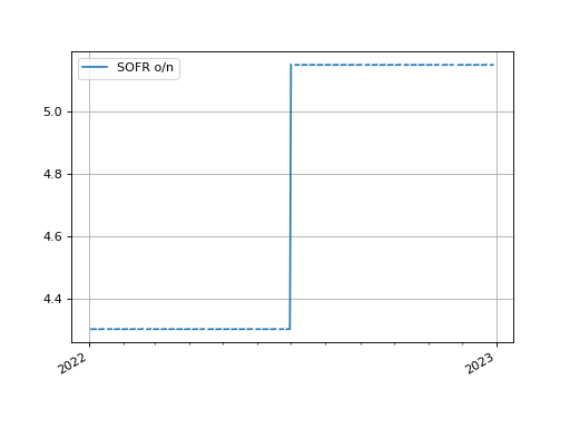
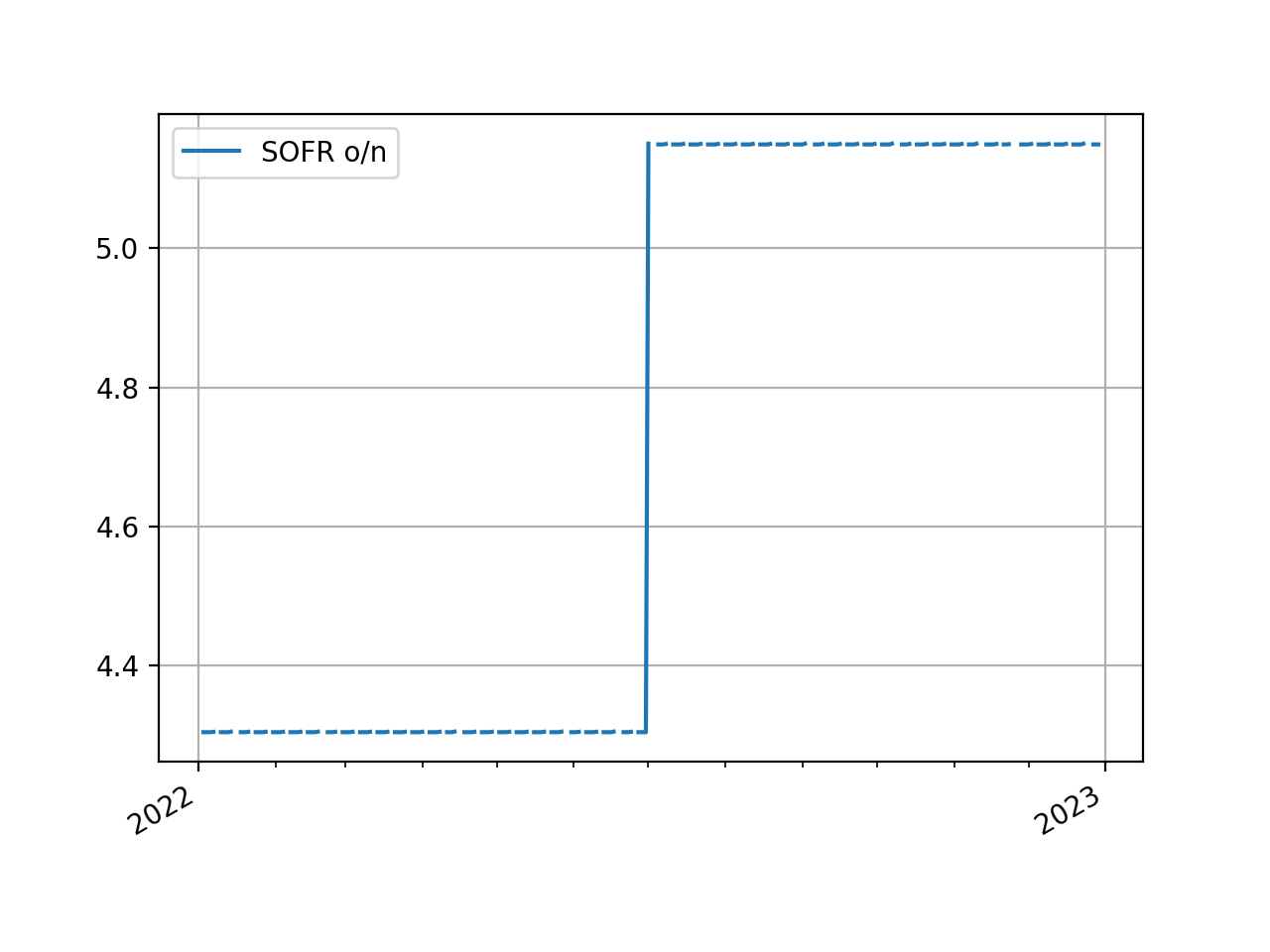
We can plot the overnight rates for the calibrated curve. This curve uses ‘log_linear’ interpolation so the overnight forward rates are constant between node dates.
In [27]: usd_curve.plot("1b", labels=["SOFR o/n"])
Out[27]:
(<Figure size 640x480 with 1 Axes>,
 <Axes: >,
 [<matplotlib.lines.Line2D at 0x11ccabb10>])
(Source code, png, hires.png, pdf)

Pricing Mechanisms#
Since rateslib is an object oriented library with object associations we give detailed instructions of the way in which the associations can be constructed in mechanisms.
The key takeway is that when you initialise and create an Instrument you can do one of three things:
Not provide any Curves (or Vol surface) for pricing upfront (
curves=NoInput(0)).Create an explicit association to pre-existing Python objects, e.g.
curves=my_curve.Define some reference to a Curves mapping with strings using
curves="my_curve_id".
If you do 1) then you must provide Curves at price
time: instrument.npv(curves=my_curve).
If you do 2) then you do not need to provide anything further at price time:
instrument.npv(). But you still can provide Curves directly, like for 1), as an override.
If you do 3) then you can provide a Solver which contains the Curves and will
resolve the string mapping: instrument.npv(solver=my_solver). But you can also provide Curves
directly, like for 1), as an override.
Best practice in rateslib is to use 3). This is the safest and most flexible approach and designed to work best with risk sensitivity calculations also.
Risk Sensitivities#
Rateslib’s can calculate delta and cross-gamma risks relative to the calibrating Instruments of a Solver. Rateslib also unifies these risks against the FX rates used to create an FXForwards market, to provide a fully consistent risk framework expressed in arbitrary currencies. See the risk framework notes.
Performance wise, because rateslib uses dual number AD upto 2nd order, combined with the appropriate analysis, it is shown to calculate a 150x150 Instrument cross-gamma grid (22,500 elements) from a calculated portfolio NPV in approximately 250ms.
Utilities#
Rateslib could not function without some utility libraries. These are often referenced in other guides as they arise and can also be linked to from those sections.
Specifically those utilities are:
Cookbook#
This is a collection of more detailed examples and explanations that don’t necessarily fall into any one category. See the Cookbook index.