
[1]:
from rateslib import *
Valuing Historical Swaps at Today’s Date#
A common operation is to want to value a swap which has an effective date in the past. To do this, the swap should not be altered in its definition but it likely requires additional pricing information supplied, in the form of fixings. See ‘Cookbook > Working with Fixings’ for more detail on this aspect.
[2]:
curve = Curve({dt(2024, 7, 3): 1.0, dt(2025, 7, 3): 0.95}, calendar="nyc")
irs = IRS(dt(2024, 6, 26), "1m", spec="usd_irs", curves=curve, fixed_rate=5.00)
This swap cant price directly because today is 3rd July and it started on 26th June and it is missing information on some of the fixings.
[3]:
try:
    irs.npv()
except ValueError as e:
    print(e)
RFRs could not be calculated, have you missed providing `fixings` or does the `Curve` begin after the start of a `FloatPeriod` including the `method_param` adjustment?
For further info see: Documentation > Cookbook > Working with fixings.
The SOFR fixings are needed for the following reference value dates in the past (as measured as of 3rd July 2024):
[4]:
get_calendar("nyc").bus_date_range(dt(2024, 6, 26), dt(2024, 7, 2))
[4]:
[datetime.datetime(2024, 6, 26, 0, 0),
 datetime.datetime(2024, 6, 27, 0, 0),
 datetime.datetime(2024, 6, 28, 0, 0),
 datetime.datetime(2024, 7, 1, 0, 0),
 datetime.datetime(2024, 7, 2, 0, 0)]
Normally these fixings would be populated by some automated data collection service or CSV file upload, but here they have been manually inserted.
[5]:
from pandas import Series
sofr_fixings = Series(
    data=[5.34, 5.34, 5.33, 5.40, 5.35],
    index=get_calendar("nyc").bus_date_range(dt(2024, 6, 26), dt(2024, 7, 2))
)
sofr_fixings
[5]:
2024-06-26    5.34
2024-06-27    5.34
2024-06-28    5.33
2024-07-01    5.40
2024-07-02    5.35
dtype: float64
The definition of the swap is altered to also input the fixings and then it is repriced with the curve, correctly, without raising errors.
[6]:
irs = IRS(dt(2024, 6, 26), "1m", spec="usd_irs", curves=curve, fixed_rate=5.0, leg2_fixings=sofr_fixings)
irs.npv()
[6]:
np.float64(113.51930516664925)
For further visibility on what rates are used to value the floating leg of the swap the fixings_table method can be used on the floating leg.
[7]:
irs.leg2.fixings_table(curve)
[7]:
| notional | dcf | rates | |
|---|---|---|---|
| obs_dates | |||
| 2024-06-26 | 0.000000e+00 | 0.002778 | 5.340000 |
| 2024-06-27 | 0.000000e+00 | 0.002778 | 5.340000 |
| 2024-06-28 | 0.000000e+00 | 0.008333 | 5.330000 |
| 2024-07-01 | 0.000000e+00 | 0.002778 | 5.400000 |
| 2024-07-02 | 0.000000e+00 | 0.002778 | 5.350000 |
| 2024-07-03 | 1.000477e+06 | 0.005556 | 5.059776 |
| 2024-07-05 | 1.000759e+06 | 0.008333 | 5.060131 |
| 2024-07-08 | 1.001181e+06 | 0.002778 | 5.059420 |
| 2024-07-09 | 1.001321e+06 | 0.002778 | 5.059420 |
| 2024-07-10 | 1.001462e+06 | 0.002778 | 5.059420 |
| 2024-07-11 | 1.001603e+06 | 0.002778 | 5.059420 |
| 2024-07-12 | 1.001743e+06 | 0.008333 | 5.060131 |
| 2024-07-15 | 1.002166e+06 | 0.002778 | 5.059420 |
| 2024-07-16 | 1.002307e+06 | 0.002778 | 5.059420 |
| 2024-07-17 | 1.002448e+06 | 0.002778 | 5.059420 |
| 2024-07-18 | 1.002588e+06 | 0.002778 | 5.059420 |
| 2024-07-19 | 1.002729e+06 | 0.008333 | 5.060131 |
| 2024-07-22 | 1.003152e+06 | 0.002778 | 5.059420 |
| 2024-07-23 | 1.003293e+06 | 0.002778 | 5.059420 |
| 2024-07-24 | 1.003434e+06 | 0.002778 | 5.059420 |
| 2024-07-25 | 1.003575e+06 | 0.002778 | 5.059420 |
Alternatively the cashflows method gives an alternative, holistic perspective.
[8]:
irs.cashflows()
[8]:
| Type | Period | Ccy | Acc Start | Acc End | Payment | Convention | DCF | Notional | DF | Collateral | Rate | Spread | Cashflow | NPV | FX Rate | NPV Ccy | ||
|---|---|---|---|---|---|---|---|---|---|---|---|---|---|---|---|---|---|---|
| leg1 | 0 | FixedPeriod | Stub | USD | 2024-06-26 | 2024-07-26 | 2024-07-30 | act360 | 0.083333 | 1000000.0 | 0.996213 | None | 5.000000 | NaN | -4166.666667 | -4150.887045 | 1.0 | -4150.887045 |
| leg2 | 0 | FloatPeriod | Stub | USD | 2024-06-26 | 2024-07-26 | 2024-07-30 | act360 | 0.083333 | -1000000.0 | 0.996213 | None | 5.136741 | 0.0 | 4280.617516 | 4264.406350 | 1.0 | 4264.406350 |
Valuing Spot Swaps at Future Dates#
The current design of rateslib targets accurate evaluation of instruments at today’s date. Valuing swaps as of future dates is something that might be required in calculations such as those for XVA or scenario analysis.
Currently rateslib does have some limited features to permit this.
As an example suppose today’s date is 3rd July 2024 and we construct an 11m IRS with a monthly frequency. A more granular Curve is constructed in this example.
[9]:
curve = Curve(
    nodes={
        dt(2024, 7, 3): 1.0,
        dt(2024, 8, 3): 1.0,
        dt(2024, 9, 3): 1.0,
        dt(2024, 10, 3): 1.0,
        dt(2024, 11, 3): 1.0,
        dt(2024, 12, 3): 1.0,
        dt(2025, 1, 3): 1.0,
        dt(2025, 2, 3): 1.0,
        dt(2025, 3, 3): 1.0,
        dt(2025, 4, 3): 1.0,
        dt(2025, 5, 3): 1.0,
        dt(2025, 6, 3): 1.0,
        dt(2025, 7, 3): 1.0,
    },
    calendar="nyc",
)
solver = Solver(
    curves=[curve],
    instruments=[
        IRS(dt(2024, 7, 3), _, spec="usd_irs", curves=curve) for _ in
        ["1m", "2m", "3m", "4m", "5m", "6m", "7m", "8m", "9m", "10m", "11m", "1y"]
    ],
    s=[5.33, 5.33, 5.315, 5.28, 5.25, 5.21, 5.17, 5.15, 5.11, 5.07, 5.04, 5.00]
)
SUCCESS: `func_tol` reached after 3 iterations (levenberg_marquardt), `f_val`: 2.4782111521459966e-12, `time`: 0.0070s
[10]:
irs = IRS(dt(2024, 7, 3), "11m", "M", spec="usd_irs", curves=curve, fixed_rate=5.04)
irs.npv()
[10]:
<Dual: -1065.843488, (b10c9_0, b10c9_1, b10c9_2, ...), [999706.0, -4301.1, -4596.4, ...]>
Today’s date as the valuation evaluation date#
Today’s date, as the evaluation date, is derived from the initial node date of the discount curve, i.e. the date at which the discount factor is necessarily set to be equal to 1.0.
The initial node date can be translated on a Curve to a date in the future as follows.
[11]:
translated_curve = curve.translate(dt(2024, 10, 15))
If the swap is then attempted to be priced with this translated Curve it will fail for the same reason as the section above - it cannot forecast rates before it starts.
[12]:
try:
    irs.npv(curves=translated_curve)
except ValueError as e:
    print(e)
RFRs could not be calculated, have you missed providing `fixings` or does the `Curve` begin after the start of a `FloatPeriod` including the `method_param` adjustment?
For further info see: Documentation > Cookbook > Working with fixings.
However, in this case the fixings are not known because 15th October 2024 is a future date. The solution is to supply a separate forecast curve and discount curve, where the forecast curve is capable of calculating the relevant rates. In this case the forecast curve is the very same curve that is created as of today’s date.
[ ]:
[13]:
irs.npv(curves=[curve, translated_curve])
[13]:
<Dual: -1830.917069, (b10c9_0, b10c9_1, b10c9_2, ...), [0.0, 0.0, 0.0, ...]>
When the cashflows are analysed, one can visually inspect that any cashflow that is paid before the initial node date of the discount curve is set to zero value. The floating rates are demonstarted here showing that the floating rates have still been correctly forecast for each FloatPeriod.
[14]:
irs.cashflows(curves=[curve, translated_curve])[12:16]
[14]:
| Type | Period | Ccy | Acc Start | Acc End | Payment | Convention | DCF | Notional | DF | Collateral | Rate | Spread | Cashflow | NPV | FX Rate | NPV Ccy | ||
|---|---|---|---|---|---|---|---|---|---|---|---|---|---|---|---|---|---|---|
| leg2 | 0 | FloatPeriod | Regular | USD | 2024-07-03 | 2024-08-05 | 2024-08-07 | act360 | 0.091667 | -1000000.0 | 0.000000 | None | 5.330000 | 0.0 | 4885.833333 | 0.00000 | 1.0 | 0.00000 |
| 1 | FloatPeriod | Regular | USD | 2024-08-05 | 2024-09-03 | 2024-09-05 | act360 | 0.080556 | -1000000.0 | 0.000000 | None | 5.304085 | 0.0 | 4272.735240 | 0.00000 | 1.0 | 0.00000 | |
| 2 | FloatPeriod | Regular | USD | 2024-09-03 | 2024-10-03 | 2024-10-07 | act360 | 0.083333 | -1000000.0 | 0.000000 | None | 5.235937 | 0.0 | 4363.280847 | 0.00000 | 1.0 | 0.00000 | |
| 3 | FloatPeriod | Regular | USD | 2024-10-03 | 2024-11-04 | 2024-11-06 | act360 | 0.088889 | -1000000.0 | 0.996894 | None | 5.109967 | 0.0 | 4542.193325 | 4528.08681 | 1.0 | 4528.08681 |
Plotting Future Value#
[20]:
import matplotlib.pyplot as plt
fig, ax = plt.subplots(1,1)

def _npv(date):
    t_curve = curve.translate(date)
    return irs.npv(curves=[curve, t_curve])

dates=[
    dt(2024, 7, 4),
    dt(2024, 8, 10),
    dt(2024, 9, 10),
    dt(2024, 10, 10),
    dt(2024, 11, 10),
    dt(2024, 12, 10),
    dt(2025, 1, 10),
    dt(2025, 2, 10),
    dt(2025, 3, 10),
    dt(2025, 4, 10),
    dt(2025, 5, 10),
    dt(2025, 6, 10),
]

ax.plot(dates, [_npv(_) for _ in dates])
[20]:
[<matplotlib.lines.Line2D at 0x1b163d8e810>]
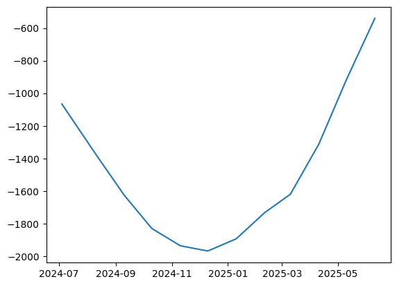
The general structure of this plot is as described in the section on ‘Cash, Collateral and Credit’ in Pricing and Trading Interest Rate Derivatives.