
Academic Curves#
Rateslib allows the construction of certain Curve classes that replicate those typically designed in academia, being parameter based. The list of such curves implemented to date are as follows:
A Nelson-Siegel curve defined by discount factors. |
|
A Nelson-Siegel-Svensson curve defined by discount factors. |
|
A Smith-Wilson style Curve defined by discount factors. |
These Curves are all _BaseCurve classes so can be used throughout the
library to interact with objects such as Instruments, Legs, Periods, etc.
They also interit _WithMutability allowing them to interact with a
Solver, for calibration.
Example#
Below we take a selection of Swedish government bond yield-to-maturities and calibrate these Curves. First we define the bonds (as priced on 9th Jan 2026). All the bonds are set to start over a year ago so the last coupon date will automatically be at an appropriate roll date.
In [1]: se_gb_args = dict(spec="se_gb", metric="ytm", curves="academic_curve")

In [2]: bonds = [
   ...:     FixedRateBond(dt(2025, 1, 1), dt(2026, 11, 12), fixed_rate=1.0, **se_gb_args),
   ...:     FixedRateBond(dt(2025, 1, 1), dt(2028, 5, 12), fixed_rate=0.75, **se_gb_args),
   ...:     FixedRateBond(dt(2025, 1, 1), dt(2029, 11, 12), fixed_rate=0.75, **se_gb_args),
   ...:     FixedRateBond(dt(2025, 1, 1), dt(2031, 5, 12), fixed_rate=0.125, **se_gb_args),
   ...:     FixedRateBond(dt(2025, 1, 1), dt(2032, 6, 1), fixed_rate=2.25, **se_gb_args),
   ...:     FixedRateBond(dt(2025, 1, 1), dt(2033, 11, 11), fixed_rate=1.75, **se_gb_args),
   ...:     FixedRateBond(dt(2025, 1, 1), dt(2035, 5, 11), fixed_rate=2.25, **se_gb_args),
   ...:     FixedRateBond(dt(2025, 1, 1), dt(2039, 3, 30), fixed_rate=3.5, **se_gb_args),
   ...:     FixedRateBond(dt(2025, 1, 1), dt(2045, 11, 24), fixed_rate=0.5, **se_gb_args),
   ...: ]
   ...:

In [3]: ytms = [2.018, 2.088, 2.267, 2.42, 2.522, 2.659, 2.798, 2.98, 3.078]
Now we define the Curves. We use the same id each time
so that the Solver
provides a consistent Curve mapping each time with the above Instruments.
In [4]: ns = NelsonSiegelCurve(
   ...:     dates=(dt(2026, 1, 9), dt(2046, 1, 10)),
   ...:     parameters=(0.01, 0.01, 0.05, 1.0),
   ...:     id="academic_curve",
   ...: )
   ...:

In [5]: nss = NelsonSiegelSvenssonCurve(
   ...:     dates=(dt(2026, 1, 9), dt(2046, 1, 10)),
   ...:     parameters=(0.01, 0.01, 0.05, 1.0, 0.05, 1.0),
   ...:     id="academic_curve",
   ...: )
   ...:

In [6]: sw = SmithWilsonCurve(
   ...:     nodes={
   ...:         dt(2026, 1, 9): 0.125,   #  <-- this is the alpha value
   ...:         **{b.leg1.schedule.termination: 0.1 for b in bonds},
   ...:     },
   ...:     ufr=4.2,
   ...:     id="academic_curve",
   ...: )
   ...:
Next we will design a factory function to calibrate these curves and return each relevant
Solver.
In [7]: def solver_factory(curve) -> Solver:
   ...:     return Solver(
   ...:         curves=[curve],
   ...:         instruments=bonds,
   ...:         s=ytms,
   ...:         func_tol=1e-5,
   ...:         conv_tol=1e-6,
   ...:         algorithm="levenberg_marquardt",
   ...:         ini_lambda=(2000, 0.5, 3),
   ...:     )
   ...:
Notice that we added some convergence parameters that are, otherwise, rarely seen in the
documentation. This is becuase these academic curves can be very sensitive to the
parameters. These func_tol and conv_tol are far less restrictive than usual and so the
iteration is much more likely to stop in and around the neighbourhood of some solution.
For failed iterations it is a fair bet that loosening the tolerances in order to stop earlier
might solve those problems.
Additionally the ini_lambda parameters have also been changed. Normally the default is
(1000, 0.25, 2) which says that the damping parameter starts out at 1000, and after a
successful iteration is reduced to 0.25x its value or is doubled after a failed iteration.
This provides a reasonable transition from the very slow, but stable, “gradient_descent”
algorithm to the much faster, but potentially unstable, “gauss_newton” algorithm. The updated
values are more conservative and less likely to lead to instability, they read that the
damping parameter starts at 2000 and after a successful iteration is halved, but after a failed
iteration will treble.
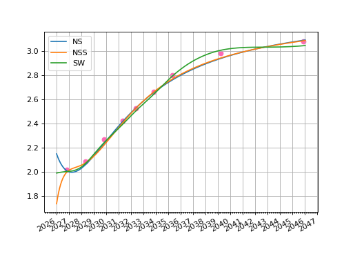
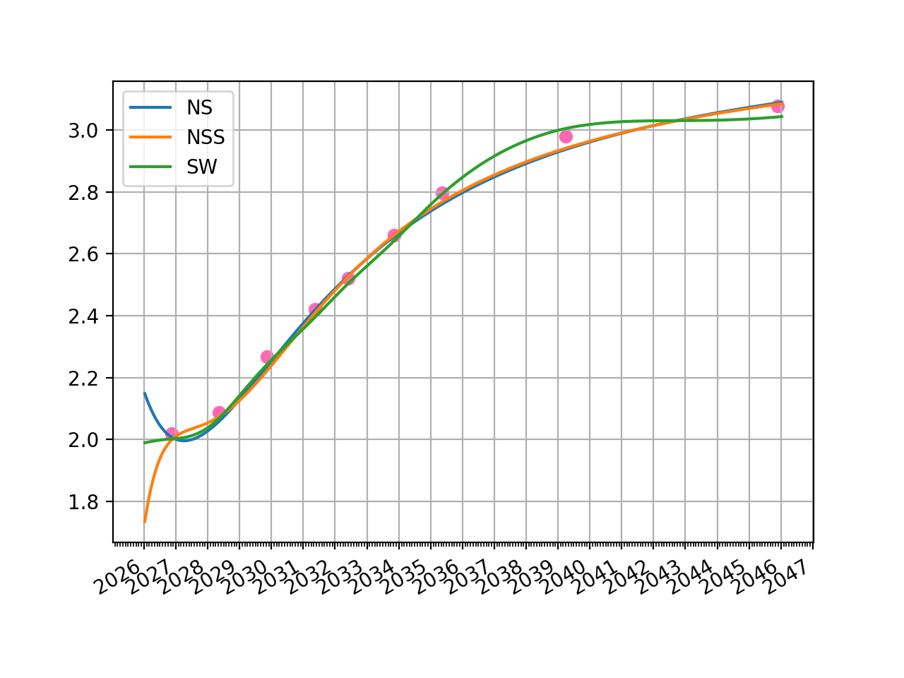
We can now calibrate the Curves and plot their zero rates.
In [8]: ns_solver = solver_factory(ns)
SUCCESS: `conv_tol` reached after 19 iterations (levenberg_marquardt), `f_val`: 0.007929630704008078, `time`: 0.0708s

In [9]: nss_solver = solver_factory(nss)
SUCCESS: `conv_tol` reached after 26 iterations (levenberg_marquardt), `f_val`: 0.006765836271071866, `time`: 0.1107s

In [10]: sw_solver = solver_factory(sw)
SUCCESS: `func_tol` reached after 30 iterations (levenberg_marquardt), `f_val`: 4.329491986569285e-06, `time`: 0.3193s

In [11]: fig, ax, lines = ns.plot("Z", comparators=[nss, sw], labels=["NS", "NSS", "SW"])

In [12]: ax.scatter(x=[_.leg1.schedule.termination for _ in bonds], y=ytms, c='hotpink')
Out[12]: <matplotlib.collections.PathCollection at 0x13c5e2cf0>
(Source code, png, hires.png, pdf)
