Less Liquid RFR Curves (MXN, COP)#

Less liquid RFR Curve building follows the same principles as demonstrated in Standard Liquid RFR Curves, except data availability might be sparser and obviously the Instruments must be chosen to match local conventions.

Key Points

Standard configuration for Curve setup.

Minor modifications for the MXN market.

Example Frameworks#

Due to data availability this example uses standard par tenor MXN F-TIIE OIS quotes as the Instruuments.

MXN swaps have an unconventional frequency expressed in 28 calendar day periods. Rateslib handles this natively as part of its Frequency framework.

Warning

In practice, MXN IRS are referred to in ‘months’ assuming ‘one-month’ is a single 28-day (or 4-week) period. This gives 13 months per year and, for example a 130-month swap would be interpreted as being the 10-year swap. Rateslib does not tolerate this colloquial definition and requires a more precise tenor to be specified. In this case 130-month is required to be entered either as “3640D” or “520W”, and the frequency is set under the spec as “28d” (equivalent to “4W”).

Data

First, load (from source) the market data for each chosen tenor of the Curve and establish the relevant dates of construction. The below code also determines the appropriate maturity of each tenor under the market calendar.

In [1]: data = DataFrame({
   ...:     "Term": ["4W", "8W", "12W", "24W", "36W", "52W", "104W", "156W", "208W", "260W", "364W", "520W", "624W", "780W", "1040W", "1560W"],
   ...:     "Rate": [7.02, 7.017, 7.015, 6.99, 6.955, 6.965, 7.155, 7.351, 7.515, 7.645, 7.855, 8.086, 8.21, 8.355, 8.48, 8.44],
   ...: })
   ...: 

In [2]: today = dt(2025, 1, 16)

In [3]: spot = get_calendar("mex").lag_bus_days(today, 2, False)

In [4]: data["Termination"] = [add_tenor(spot, _, "F", "mex") for _ in data["Term"]]

Curve Design

In order to create a perfectly solvable curve, the chosen nodes will be assigned as the maturity of each Instrument.

In [5]: ftiie = Curve(
   ...:     id="ftiie",
   ...:     convention="Act360",                          # <- important to match F-TIIE convention
   ...:     calendar="mex",                               # <- important to match F-TIIE convention
   ...:     interpolation="spline",
   ...:     nodes={
   ...:         today: 1.0,                               # <- this is today's DF,
   ...:         **{_: 1.0 for _ in data["Termination"][:-1]},  # <- every instrument node but the last
   ...:         **{data["Termination"].iloc[-1] + timedelta(days=10): 1.0},  # <- avoid spline end warnings
   ...:     }
   ...: )
   ...: 

Calibration with Solver

The final step puts the Curve and the Instruments together, mutating the Curve to match the rates: s.

In [6]: solver = Solver(
   ...:     curves=[ftiie],
   ...:     instruments=[IRS(spot, _, spec="mxn_irs", curves="ftiie") for _ in data["Termination"]],
   ...:     s=data["Rate"],
   ...:     instrument_labels=data["Term"],
   ...:     id="mx_rates",
   ...: )
   ...: 
SUCCESS: `func_tol` reached after 7 iterations (levenberg_marquardt), `f_val`: 8.248747663025201e-16, `time`: 0.9886s

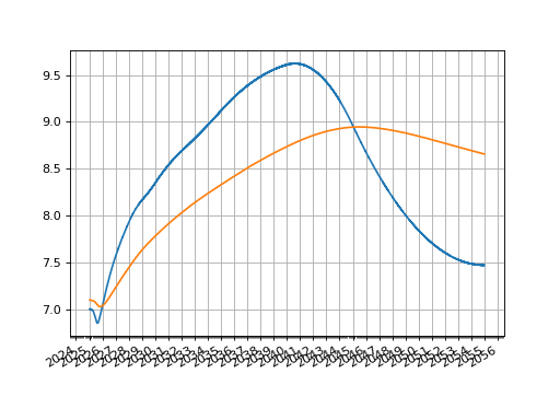
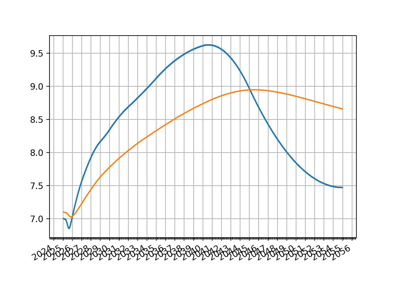
Then plotting either the O/N rates or the zero rates:

ftiie.plot("1b")
ftiie.plot("Z")

(Source code, png, hires.png, pdf)

Less Liquid RFR Curves (MXN, COP)#

Example Frameworks#

This Page