
Standard Liquid RFR Curves (USD, GBP, CAD, CHF, JPY)#
This example will discuss curve building standards for liquid RFR markets like USD, GBP, CAD, CHF, JPY. Less liquid markets like INR domestic onshore, MXN and COP for example follow the same principles but more nunaced choices of instruments may be required to suit available data.
Key Points
Standard configuration for Curve setup.
Differences between data consumers and market makers.
Advanced tinkering of convergence and Curve interpolation.
Alternative Construction Frameworks#
The advantage of these markets is that there is sufficiently granular data to construct a Curve with day-to-day consistent inputs. In this framework we choose standard tenors only to construct the Curve, and consume published data for those rates.
This is an advantage in terms of minimising on going maintenance and simplifying the setup. The following curve is constructed in six lines of code, and is replicable without fail on any day of the year.
Data
First, load (from source) the market data for each chosen tenor of the Curve and establish the relevant dates of construction. The below code also determines the appropriate maturity of each tenor under the market calendar.
In [1]: data = DataFrame({
   ...:     "Term": ["1W", "2W", "3W", "1M", "2M", "3M", "4M", "5M", "6M", "7M", "8M", "9M", "10M", "11M", "12M", "18M", "2Y", "3Y", "4Y", "5Y", "6Y", "7Y", "8Y", "9Y", "10Y", "12Y", "15Y", "20Y", "25Y", "30Y", "40Y"],
   ...:     "Rate": [5.309,5.312,5.314,5.318,5.351,5.382,5.410,5.435,5.452,5.467,5.471,5.470,5.467,5.457,5.445,5.208,4.990,4.650,4.458,4.352,4.291,4.250,4.224,4.210,4.201,4.198,4.199,4.153,4.047,3.941,3.719],
   ...: })
   ...:

In [2]: today = dt(2023, 9, 27)

In [3]: spot = get_calendar("nyc").lag_bus_days(today, 2, False)

In [4]: data["Termination"] = [add_tenor(spot, _, "MF", "nyc") for _ in data["Term"]]
Curve Design
In order to create a perfectly solvable curve, the chosen nodes will be assigned as the maturity of each Instrument.
In [5]: sofr = Curve(
   ...:     id="sofr",
   ...:     convention="Act360",                          # <- important to match SOFR convention
   ...:     calendar="nyc",                               # <- important to match SOFR convention
   ...:     interpolation="log_linear",
   ...:     nodes={
   ...:         today: 1.0,                               # <- this is today's DF,
   ...:         **{_: 1.0 for _ in data["Termination"]},  # <- every instrument node
   ...:     }
   ...: )
   ...:
Calibration with Solver
The final step puts the Curve and the Instruments together, mutating the Curve to match the rates: s.
In [6]: solver = Solver(
   ...:     curves=[sofr],
   ...:     instruments=[IRS(spot, _, spec="usd_irs", curves="sofr") for _ in data["Termination"]],
   ...:     s=data["Rate"],
   ...:     instrument_labels=data["Term"],
   ...:     id="us_rates",
   ...: )
   ...:
SUCCESS: `func_tol` reached after 6 iterations (levenberg_marquardt), `f_val`: 9.815194353211927e-12, `time`: 0.1502s
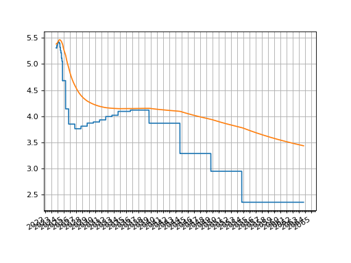
Then plotting either the O/N rates or the zero rates:
sofr.plot("1b")
sofr.plot("Z")
(Source code, png, hires.png, pdf)

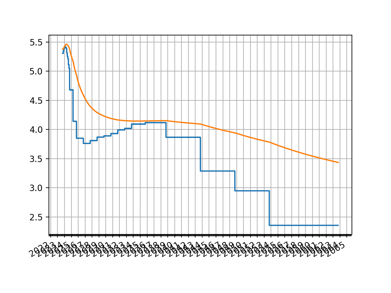
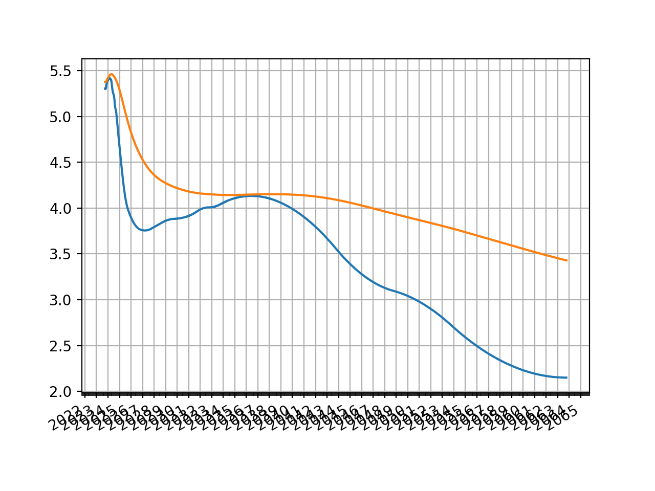
The most common tweak that one might make to this Curve is to change its interpolation style. A very simple approach is to use “spline” which applies a log-cubic spline over discount factors across the whole curve.
The t argument can also be used which specifies using a
spline only for a section of the Curve resulting in mixed interpolation.
All else remains the same.
Explicit examples of this are demonstrated in ‘Pricing and Trading Interest Rate Derivatives: Single Currency Curve Example’
sofr = Curve(
    id="sofr",
    convention="Act360",
    calendar="nyc",
    interpolation="spline",
    nodes={
        today: 1.0,
        **{_: 1.0 for _ in data["Termination"][:-1]},
        dt(2063, 10, 7): 1.0,  # <- avoid end spline warning
    }
)
(Source code, png, hires.png, pdf)

The difference between a data-consumer and market-maker approach is that a market-maker usually creates or provides their own data to construct their Curve. This allows much more flexibility, and subjectivity, in construction choices, and also more complexity. Essentially it means that the market-maker chooses their Instruments and goes about creating the data to suit that approach.
There is not one standard approach but there are some general principles that are often employed:
Curves are expected to be flat and jump on central bank effective dates at the ultra short end. Here we use ‘log_linear’
interpolationto control this.STIR Futures markets provide data at the short end of the Curve, instruments are chosen that reflect their prices. We assume that convexity adjustments are pre-processed and so the rates provided to the Instruments are swap-rate equivalent. For a framework that explicitly discusses this see Building with STIR Convexity Adjustments.
Medium term and longer term rates are derived from par tenor swap Instruments and use a log-cubie spline type interpolation to reflect sparser data. Here we configure mixed interpolation by choosing our
tknot sequence.
Data
This data is similar to the previous but amended to account for specific STIR futures periods with swap-equivalent rates.
In [7]: data = DataFrame({
   ...:     "Term": [
   ...:         "ON", "1V23", "1X23", "1Z23", "1F24", "1G24", "1H24", "1J24", "1K24", "1M24",
   ...:         "Z23", "H24", "M24", "U24", "Z24", "H25", "M25", "U25", "Z25", "H26", "M26", "U26",
   ...:         "4Y", "5Y", "6Y", "7Y", "8Y", "9Y", "10Y", "12Y", "15Y", "20Y", "25Y", "30Y", "40Y",
   ...:     ],
   ...:     "Rate": [
   ...:         5.31, 5.307, 5.353, 5.387, 5.409, 5.421, 5.408, 5.387, 5.307, 5.251,
   ...:         5.447, 5.372, 5.180, 4.913, 4.588, 4.293, 4.084, 3.969, 3.894, 3.838, 3.801, 3.782,
   ...:         4.458, 4.352, 4.291, 4.250, 4.224, 4.210, 4.201, 4.198, 4.199, 4.153, 4.047, 3.941, 3.719
   ...:     ],
   ...: })
   ...:
Dates
As of our Curve build date (27th Sep 2023) we need to know the FED effective dates and some relevant IMM dates. Beyond these we will use par tenor swap dates as the node dates.
In [8]: today = dt(2023, 9, 27)

In [9]: spot = get_calendar("nyc").lag_bus_days(today, 2, False)

In [10]: IMM1 = ["V23", "X23", "Z23", "F24", "G24", "H24", "J24", "K24", "M24"]

In [11]: IMM3 = ["Z23", "H24", "M24", "U24", "Z24", "H25", "M25", "U25", "Z25", "H26", "M26", "U26", "Z26"]

In [12]: PAR = ["4Y", "5Y", "6Y", "7Y", "8Y", "9Y", "10Y", "12Y", "15Y", "20Y", "25Y", "30Y", "40Y"]

In [13]: fed = [dt(2023, 11, 2), dt(2023, 12, 14), dt(2024, 2, 1), dt(2024, 3, 21), dt(2024, 5, 2)]

In [14]: imm = [get_imm(code=_) for _ in IMM3[2:]]

In [15]: par = [add_tenor(spot, _, "MF", "nyc") for _ in PAR]
Curve Configuration
We use the above dates and subjectively opt that the spline interpolation , controlled by
the knots t begins at the end of the 10th quarterly IMM contract contract.
In [16]: sofr = Curve(
   ....:     id="sofr",
   ....:     convention="Act360",                          # <- important to match SOFR convention
   ....:     calendar="nyc",                               # <- important to match SOFR convention
   ....:     interpolation="log_linear",
   ....:     nodes={
   ....:         today: 1.0,                               # <- this is today's DF,
   ....:         **{_: 1.0 for _ in fed},                  # <- FED effective dates,
   ....:         **{_: 1.0 for _ in imm},                  # <- 3M IMM end dates,
   ....:         **{_: 1.0 for _ in par},                  # <- Par swap maturities
   ....:     },
   ....:     t = [
   ....:         get_imm(code="M26"), get_imm(code="M26"), get_imm(code="M26"), get_imm(code="M26"),
   ....:         get_imm(code="U26"),
   ....:         get_imm(code="Z26"),
   ....:         *par[:-1],
   ....:         dt(2063, 10, 7), dt(2063, 10, 7), dt(2063, 10, 7), dt(2063, 10, 7)
   ....:     ]
   ....: )
   ....:
Calibration with Solver
We now calibrate, targeting the 3M-IMM futures rates and the par swap rates.
The 1M-IMM futures and the O/N rate serve as regularizers to constrain the Curve in case
the number of nodes (i.e. from the FED effective dates) are large. This is controlled
by the weights parameter significantly reducing the importance of these Instruments.
In [17]: solver = Solver(
   ....:     curves=[sofr],
   ....:     instruments=[
   ....:         IRS(today, "1b", spec="usd_irs", curves="sofr"),    #  <- O/N rate
   ....:         *[                                                  # <-  1M-IMM rates x 9
   ....:             STIRFuture(get_imm(code=_, definition="som"), "1m", spec="usd_stir1", curves="sofr", metric="rate")
   ....:             for _ in IMM1
   ....:         ],
   ....:         *[                                                  # <-  3M-IMM rates x 12
   ....:             STIRFuture(get_imm(code=IMM3[i]), get_imm(code=IMM3[i+1]), spec="usd_stir", curves="sofr", metric="rate")
   ....:             for i in range(12)
   ....:         ],
   ....:         *[                                                  # <-  Par swap rates x 13
   ....:             IRS(spot, _, spec="usd_irs", curves="sofr") for _ in PAR
   ....:         ]
   ....:     ],
   ....:     s=data["Rate"],
   ....:     weights=[1e-5]*10 + [1.0]*25,
   ....:     func_tol=1e-7,
   ....:     conv_tol=1e-8,
   ....: )
   ....:
SUCCESS: `func_tol` reached after 8 iterations (levenberg_marquardt), `f_val`: 2.6140100348617698e-08, `time`: 0.1387s
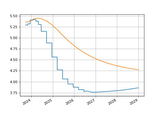
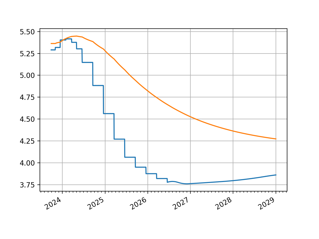
The graph looks broadly similar after the first five years.
sofr.plot("1b", right=dt(2029, 1, 1))
sofr.plot("Z", right=dt(2029, 1, 1))
(Source code, png, hires.png, pdf)

Alternatives
Employing different Instruments, using pseudo-Instruments as regularizers, changing the node dates, or the knot dates for the spline, or designing custom-Instruments to act as penalty function regularizers are all possible designs that market-makers might typically employ. For some further analysis, anecdotes of real trading and examples of these sorts of considerations see Pricing and Trading Interest Rate Derivatives: A Practical Guide to Swaps.
Bloomberg’s SWPM Curve is (under default settings) no more than a log-linearly interpolated Curve using par tenors as the node-dates. I.e. it matches the data consumer type Curve already demonstrated in these tabs. However, for legacy reasons the page giving a specific example of this is still available.