Dense Liquid Bond Curves (EUR, GBP, USD)

This example will discuss curve building standards for liquid bond markets with many actively traded bonds as data points.

Key Points

• Standard configuration for Curve setup.

• Consideration for using academic, parameter based Curves.

General SetupSolver Weights

Data

We have acquired a list of 69 UK gilt prices from a retail broker with their maturities. The accuracy of these prices may be dubious and we assume that all of them are currently settling within a regular coupon period (not a short or long stub). The data is displayed below:

In [1]: df
Out[1]: 
     Maturity  Coupon  Clean Price
0  2026-01-30    0.12        99.90
1  2026-07-22    1.50        98.93
2  2026-10-22    0.38        97.77
3  2027-01-29    4.12       100.43
4  2027-03-07    3.75       100.08
..        ...     ...          ...
64 2063-10-22    4.00        81.51
65 2065-07-22    2.50        56.49
66 2068-07-22    3.50        73.00
67 2071-10-22    1.62        41.10
68 2073-10-22    1.12        32.46

[69 rows x 3 columns]

To this DataFrame we can add our Instrument object and some easy to calculate metrics:

In [2]: df["Bond"] = [
   ...:     FixedRateBond(
   ...:         effective=dt(2025, 1, 1),
   ...:         termination=t,
   ...:         spec="uk_gb",
   ...:         fixed_rate=c,
   ...:         curves="uk_gb_curve",
   ...:         metric="clean_price"
   ...:     ) for (t, c) in zip(df["Maturity"], df["Coupon"])
   ...: ]
   ...: 

In [3]: df["Accrued"] = [b.accrued(settlement=dt(2026, 1, 19)) for b in df["Bond"]]

In [4]: df["YTM"] = [b.ytm(price=p, settlement=dt(2026, 1, 19)) for (b, p) in zip(df["Bond"], df["Clean Price"])]

In [5]: df["Risk"] = [b.duration(ytm=y, settlement=dt(2026, 1, 19)) for (b, y) in zip(df["Bond"], df["YTM"])]

In [6]: df
Out[6]: 
     Maturity  Coupon  Clean Price                               Bond  Accrued  YTM  Risk
0  2026-01-30    0.12        99.90  <rl.FixedRateBond at 0x12dba6d50>     0.06 3.50  0.03
1  2026-07-22    1.50        98.93  <rl.FixedRateBond at 0x12dba69f0>    -0.01 3.64  0.49
2  2026-10-22    0.38        97.77  <rl.FixedRateBond at 0x12dba6330>     0.09 3.39  0.73
3  2027-01-29    4.12       100.43  <rl.FixedRateBond at 0x12dba61b0>     1.95 3.69  1.00
4  2027-03-07    3.75       100.08  <rl.FixedRateBond at 0x12dba5fd0>     1.39 3.67  1.10
..        ...     ...          ...                                ...      ...  ...   ...
64 2063-10-22    4.00        81.51  <rl.FixedRateBond at 0x12d9666f0>     0.98 5.11 14.23
65 2065-07-22    2.50        56.49  <rl.FixedRateBond at 0x12d9660f0>    -0.02 5.05 11.13
66 2068-07-22    3.50        73.00  <rl.FixedRateBond at 0x12d967050>    -0.03 5.05 13.61
67 2071-10-22    1.62        41.10  <rl.FixedRateBond at 0x12d965b50>     0.40 4.83  9.52
68 2073-10-22    1.12        32.46  <rl.FixedRateBond at 0x12d965910>     0.28 4.67  8.50

[69 rows x 7 columns]

Curves

We will build a Curve and, as comparison, an academic NelsonSiegelCurve. The choice of the node dates on the Curve are subjectively chosen suit the local market and available data.

In [7]: curve = Curve(
   ...:     id="uk_gb_curve",
   ...:     calendar="ldn",
   ...:     convention="act365f",
   ...:     interpolation="spline",
   ...:     nodes={
   ...:          dt(2026, 1, 16): 1.0,
   ...:          **{add_tenor(dt(2026, 1, 16), _, "None"): 1.0
   ...:             for _ in ["4m", "1y", "2y", "3y", "4y", "5y", "7y", "10y", "15y", "20y", "25y", "30y", "40y", "50y"]}
   ...:     }
   ...: )
   ...: 

In [8]: ns = NelsonSiegelCurve(
   ...:     id="uk_gb_curve",
   ...:     calendar="ldn",
   ...:     convention="act365f",
   ...:     dates=(dt(2026, 1, 16), dt(2076, 1, 16)),
   ...:     parameters=[0.01, 0.01, 0.01, 0.5],
   ...: )
   ...: 

Calibration and Solver

We will setup a solver factory in order to create an individual :class:~rateslib.solver.Solver` for each Curve passed as an argument - in order to eliminate repeated code. The convergence tolerances here are fairly loose to promote early stopping and avoid failed iterations.

In [9]: def solver_factory(c):
   ...:     return Solver(
   ...:         curves=[c],
   ...:         instruments=df["Bond"],
   ...:         s=df["Clean Price"],
   ...:         conv_tol=1e-5,
   ...:         ini_lambda = (10000, 0.5, 3)
   ...:     )
   ...: 

In [10]: c_solver = solver_factory(curve)
SUCCESS: `conv_tol` reached after 7 iterations (levenberg_marquardt), `f_val`: 17.453656807813022, `time`: 0.1070s

In [11]: ns_solver = solver_factory(ns)
SUCCESS: `conv_tol` reached after 13 iterations (levenberg_marquardt), `f_val`: 63.557789371285125, `time`: 0.2247s

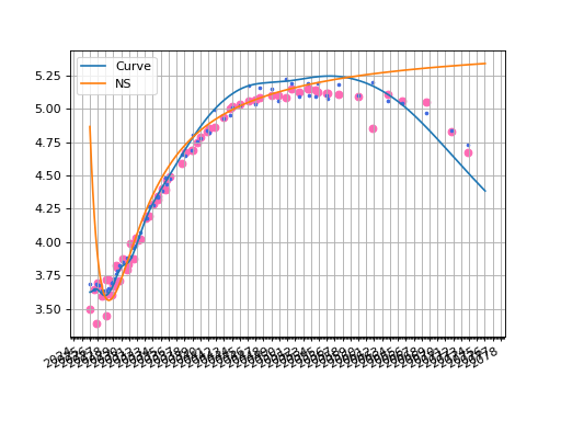
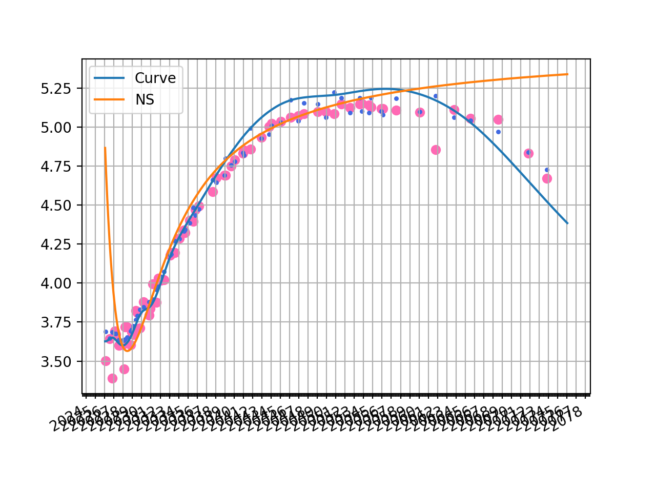
The plotted zero rate curve alongside scattered YTMs is visible below. Additionally, we show the corresponding YTMs for each bond calculated with the Curve in matching color.

fig, ax, lines = curve.plot("Z", comparators=[ns], labels=["Curve", "NS"])
ax.scatter(df["Maturity"], df["YTM"], color="hotpink")
ax.scatter(df["Maturity"], [b.rate(solver=c_solver, metric="ytm") for b in df["Bond"]], color="royalblue", s=5)
plt.show()

(Source code, png, hires.png, pdf)